💡AP Physics C: E&M
💡AP Physics C: E&M
FRQ 1 – Mathematical Routines
Unit 8: Electric Charges, Fields, and Gauss's Law
Practice FRQ 1 of 201/20
1. A solid insulating sphere of radius is centered inside a thin, conducting spherical shell with inner radius and outer radius , as shown in Figure 1. The insulating sphere has a uniform volume charge density . The conducting shell has a net charge . The system is in electrostatic equilibrium and is surrounded by air. The permittivity of air may be taken as .
Figure 1. Insulating sphere centered inside a conducting spherical shell (electrostatic equilibrium).
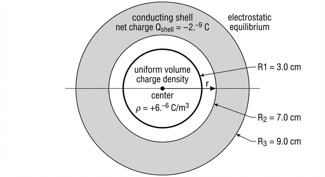
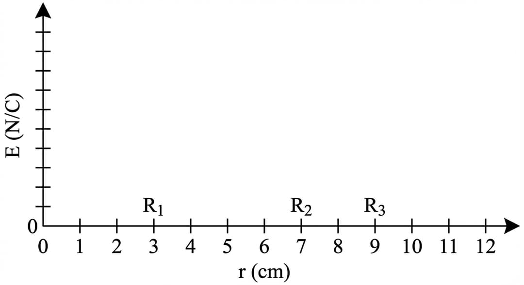
Figure 2. Axes for graphing electric-field magnitude E versus radial distance r.
A.
i. Using Gauss's law, derive an expression for the magnitude of the electric field as a function of radial distance for the region . Express your answer in terms of , , , and physical constants, as appropriate.
ii. Derive an expression for the net charge on the inner surface of the conducting shell and the net charge on the outer surface of the conducting shell. Express your answers in terms of , , , and physical constants, as appropriate. Begin your derivation by writing a fundamental physics principle or an equation from the reference information.
iii. On the axes shown in Figure 2, sketch a graph of as a function of from to a position that is outside the outer surface of the shell.
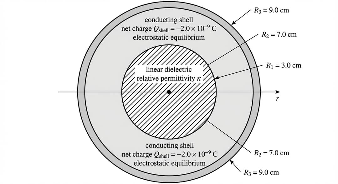
A dielectric material with relative permittivity completely fills the region , as shown in Figure 3. The free charge density in the sphere remains uniform and equal to , and the conducting shell still has net charge .
B. Derive an expression for the magnitude of the electric field as a function of for the region with the dielectric present. Express your answer in terms of , , , and physical constants, as appropriate. Begin your derivation by writing a fundamental physics principle or an equation from the reference information.
Figure 3. Same geometry as Figure 1, but the inner sphere region is a linear dielectric (relative permittivity κ).