Sometimes, the least squares regression model may not be the best for representing a data set. We’re going to list some reasons why. While we briefly introduced them in section 2.4, we'll go into further detail here.
Influential Points
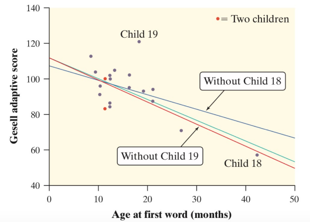
An influential point is a point that when added, significantly changes the regression model, whether by affecting the slope, y-intercept, or correlation. There are two types: outliers and high-leverage points, which are both shown in this graph.

Outliers
An outlier is a point in which the y-value is far away from the rest of the points, that is, it has a high-magnitude residual. These points heavily reduce the correlation of the scatterplot and can occasionally change the y-intercept of a regression line. Child 19 on the scatterplot above is an outlier.
High-Leverage Points
A high-leverage point is a point at which the x-value is far away from the rest of the points. These points pull the regression line towards this point, and thus can significantly change the slope of the line. It can occasionally change the y-intercept of a regression line. Child 18 on the scatterplot above is a high-leverage point.
Overall, it's crucial to identify influential points in a regression model because they can have a large impact on the estimates of the model parameters and the overall fit of the model. If an influential point is an outlier, it may be appropriate to exclude it from the model because it may not be representative of the underlying pattern in the data. If an influential point is a high-leverage point, it may be worth considering whether the model is appropriate for the data or if a different model would be more suitable.
Transforming Data and Nonlinear Regression
Sometimes, a linear model is not a good fit for a set of data, and thus it is better to use a nonlinear model. The types that we have to know for this class are exponential and power regression models. (There is also polynomial regression, but that requires knowledge of linear algebra, which is beyond the scope of this course.)
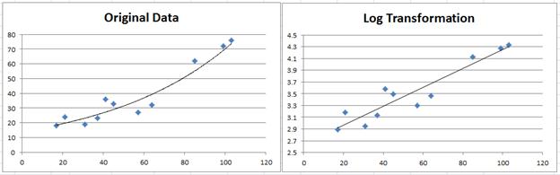
To use exponential and power regression models, it is usually necessary to transform the data to linearize it. This involves applying a function to the predictor and/or response variables in order to transform them into a form that is more suitable for linear regression. For example, the logarithmic transformation is often used to linearize exponential data, while the square root or logarithmic transformation is often used to linearize power data.
Don't worry, though! Most calculators have options to automatically calculate this for you.
Exponential Models
Exponential models have the form ŷ=ab^x, where a and b are constants and x is the explanatory variable. In order to fit an exponential model using linear regression, it is necessary to transform the data so that the relationship between the transformed response variable and the predictor variable is linear.
To do this, you can take the natural logarithm of both sides of the exponential model equation. This gives you ln(ŷ) = ln(a) + ln(b)x. The relationship between ln(ŷ) and x is now linear, so you can fit a linear regression model to the transformed data. The y-intercept of the model will be equal to ln(a), and the slope will be equal to ln(b).
This means that the relationship between ln(ŷ) and x is linear, so we find the LSRL of this transformed data with the y-intercept being a* and the slope being b*. To find a and b, we use:

Power Models
Power models have the form ŷ=ax^b. Like exponential models, we also take the natural logarithm of both sides, and with manipulation, we get ln(ŷ) = ln(a) + bln(x). This time, the relationship between ln(ŷ) and ln(x) is linear. With the LSRL of the transformer data again having y-intercept a* and slope b*, we have:
How Can I Tell, Then?
When evaluating which transformation to use in an exponential or power regression model, it's important to consider both the residual plots of the transformed data and the R^2 value. We pick the right model by seeing whether the residuals are randomly scattered and not curved and also whether the R^2 is close to 1.
By the way, the R^2 is interpreted as the percent of variation in the response variable that can be explained by a power/exponential model relative to the explanatory variable, which is very similar to its linear counterpart. If the conditions above aren’t met, then there may be another model that may work that we haven’t learned or there are influential points skewing the data set, which is more likely!
To summarize, if our data appears to be an exponential model, we need to take the natural log (or any other base log) of our y coordinates. If our data appears to be a power model, such as a quadratic or cubic function, we need to take the log of both our x and y coordinates.
🎥 Watch: AP Stats - Exploring Two-Variable Data
Practice Problem
You are a statistician working for a company that manufactures and sells a certain type of light bulb. The company wants to understand how the price of the light bulbs affects the number of units sold. To do this, you collect data on the number of units sold and the price of the light bulbs for a sample of 50 different stores.
You begin by performing a linear regression on the data and find that the model has a poor fit, with a low R-squared value. You decide to try transforming the data by taking the natural logarithm of the number of units sold, and then performing a linear regression on the transformed data.
You find that the transformed data has a better fit, with a higher R-squared value. The equation of the transformed model is:
ln(units sold) = 0.5 * ln(price) + 2
You want to transform the model back to its original form so that you can make predictions in terms of the original variables. To do this, you can use the following formula:
units sold = e^(b * price^a), where a and b are constants.
Using the equation of the transformed model, find the values of a and b in the original model.
Hint: Remember that the natural logarithm of a number is the exponent to which the base e must be raised to get that number. For example, ln(2) = 0.69, because e^0.69 = 2.
Answer
First, we need to rewrite the equation of the transformed model in terms of the original variables. Since ln(units sold) is equal to 0.5 * ln(price) + 2, we can rewrite this equation as:
ln(units sold) = ln(price^0.5) + 2
Using the property of logarithms that ln(a^b) = b * ln(a), we can rewrite the equation as:
ln(units sold) = 0.5 * ln(price) + 2
Then, we can use the formula for the original model to find the values of a and b. Setting a equal to 0.5 and b equal to e^2, we get:
units sold = e^(2 * price^0.5)
Therefore, the values of a and b in the original model are a = 0.5 and b = e^2.
Vocabulary
The following words are mentioned explicitly in the College Board Course and Exam Description for this topic.Term | Definition |
|---|---|
coefficient of determination | The value r², which represents the proportion of variation in the response variable that is explained by the explanatory variable in the regression model. |
correlation | A numerical measure (r) that describes the strength and direction of a linear relationship between two variables, ranging from -1 to 1. |
high-leverage point | A point in regression that has a substantially larger or smaller x-value than other observations in the dataset. |
influential points | Points in a regression that, when removed, substantially change the relationship between variables, such as the slope, y-intercept, or correlation. |
least-squares regression line | A linear model that minimizes the sum of squared residuals to find the best-fitting line through a set of data points. |
natural logarithm | A mathematical transformation using the logarithm with base e, often applied to response or explanatory variables to linearize relationships. |
outlier | Data points that are unusually small or large relative to the rest of the data. |
residual | The difference between the actual observed value and the predicted value in a regression model, calculated as residual = y - ŷ. |
residual plot | A scatter plot that displays residuals on the vertical axis versus either the explanatory variable values or predicted response values on the horizontal axis, used to assess the fit of a regression model. |
slope | The value b in the regression equation ŷ = a + bx, representing the rate of change in the predicted response for each unit increase in the explanatory variable. |
transformed data set | A dataset created by applying mathematical transformations (such as logarithms or powers) to the original variables to achieve a more linear relationship. |
y-intercept | The value a in the regression equation ŷ = a + bx, representing the predicted response value when the explanatory variable equals zero. |
Frequently Asked Questions
How do I tell if a point is an outlier vs a high leverage point?
Outlier vs. high-leverage point—quick rule of thumb: - Outlier (regression outlier): a point that doesn’t follow the pattern in y. It has a large residual from the LSRL (often flagged when the studentized/standardized residual ≳ 2 or 3). It tells you the point’s y is surprising given its x (CED DAT-1.I.1). - High-leverage point: a point with an x-value far from the other x’s. It can pull the LSRL because it lies out on the x-axis (CED DAT-1.I.2). Leverage is measured by hat values; a common cutoff is much larger than the average hat value (≈ (p+1)/n), e.g. >2× that average. - Influential: a point that, if removed, substantially changes the slope/intercept/correlation (CED DAT-1.I.3). High leverage points often are influential, especially if they’re also outliers in y. You can use diagnostics (studentized residuals, hat values, Cook’s distance) to flag each: large residual → outlier; large hat → high leverage; large Cook’s D → influential. For practice and AP-aligned review see the Topic 2.9 study guide (https://library.fiveable.me/ap-statistics/unit-2/analyzing-departures-linearity/study-guide/Krgk1LYlZMysG2Etzh4W) and more problems at the Unit 2 page (https://library.fiveable.me/ap-statistics/unit-2) or practice bank (https://library.fiveable.me/practice/ap-statistics).
What's the difference between an outlier and an influential point in regression?
An outlier is a point that doesn’t follow the overall pattern and has a large residual from the LSRL—it lies far from the line vertically (CED: DAT-1.I.1). A high-leverage point has an x-value far from the other x’s (CED: DAT-1.I.2). An influential point is any observation that, if removed, substantially changes the fitted regression (slope, intercept, or r); high-leverage points and outliers are often influential but not always (CED: DAT-1.I.3). Quick checks you can use: look at residuals to spot outliers, look at x-position to spot leverage, and compare the LSRL with and without a point (or use Cook’s distance/hat values) to decide influence. This is exactly what's tested in Topic 2.9—see the study guide for examples (https://library.fiveable.me/ap-statistics/unit-2/analyzing-departures-linearity/study-guide/Krgk1LYlZMysG2Etzh4W). For more practice, try problems at (https://library.fiveable.me/practice/ap-statistics) or review Unit 2 (https://library.fiveable.me/ap-statistics/unit-2).
When do I need to transform my data before doing linear regression?
You should transform before doing linear regression when the relationship between x and y isn’t approximately linear or when the regression assumptions break down. Signs that a transform might help: - Residual plot shows a curved pattern (not random scatter) → violates linearity (CED DAT-1.J.1). - Residual spread changes with x (fanning) → unequal variance. - Residuals aren’t roughly normal (especially for inference on slope). - A few points strongly influence the fit (try transform plus check leverage/Cook’s distance). Common fixes: log(y) or log(x), square or sqrt(x), or Box–Cox. You decide by trying transforms and comparing: does the residual plot look more random, and does R² move closer to 1? If so, the transformed LSRL is a better model (CED DAT-1.J.2). Remember to back-transform predicted values into original units when you report predictions. For AP review, see the Topic 2.9 study guide (https://library.fiveable.me/ap-statistics/unit-2/analyzing-departures-linearity/study-guide/Krgk1LYlZMysG2Etzh4W) and practice problems at (https://library.fiveable.me/practice/ap-statistics).
How do I calculate a predicted value using transformed data?
If you transform data (common: ln(y) or square x) do all modeling on the transformed scale and then back-transform your prediction. Steps: 1. Transform the appropriate variable(s). Example: use ln(y) when you log-transform the response (CED DAT-1.J.1). 2. Fit the LSRL on transformed data to get â and b̂ for the model on the transformed scale (e.g., ln(y)̂ = â + b̂ x). 3. For a given x0, compute the predicted transformed response: T̂0 = â + b̂ x0. 4. Back-transform T̂0 to the original units: if T = ln(y) then ŷ = e^{T̂0}; if T = y^2 then ŷ = sqrt(T̂0). State units and context (CED: predicted response). 5. Note interpretation & limitation: a back-transformed prediction from ln(y) gives a multiplicative (geometric/median) prediction, not the original mean; for unbiased mean predictions you’d need a correction (beyond AP scope). Check residual plot and r² to confirm the transformed model is more appropriate (CED DAT-1.J.2). For more examples and practice on Topic 2.9, see the study guide (https://library.fiveable.me/ap-statistics/unit-2/analyzing-departures-linearity/study-guide/Krgk1LYlZMysG2Etzh4W) and many practice questions (https://library.fiveable.me/practice/ap-statistics).
I don't understand what makes a point "influential" - can someone explain this step by step?
An influential point is one that meaningfully changes your regression if you remove it. Step-by-step: 1. Look at the point on the scatterplot. Ask: is its x-value much larger/smaller than the others? If yes, it has high leverage (CED: DAT-1.I.2). 2. Fit the LSRL and check the residual for that point. A large residual = regression outlier (DAT-1.I.1). 3. If a point has both high leverage and a large residual it’s often influential, but either can be enough. 4. Test influence: remove the point and refit the LSRL. If slope, intercept, or r (or r²) changes noticeably (CED: DAT-1.I.3), the point is influential. 5. For formal checks use diagnostics (Cook’s distance, hat values, studentized residuals) in your calculator/software. Large Cook’s or hat value flags influence. On the AP exam you’ll usually identify influence by describing leverage/residual and saying how slope/correlation would change if the point were removed (Topic 2.9; see study guide: https://library.fiveable.me/ap-statistics/unit-2/analyzing-departures-linearity/study-guide/Krgk1LYlZMysG2Etzh4W). For extra practice, try problems at (https://library.fiveable.me/practice/ap-statistics).
What's the formula for finding high leverage points?
The usual numeric way to identify high-leverage points is the hat (leverage) value hi. For simple linear regression (one x), the formula is hi = 1/n + (x_i − x̄)² / Σ(x_j − x̄)². Hi measures how far an observation’s x is from the mean x; larger hi = more leverage. A common rule of thumb: in simple linear regression a point is “high leverage” if hi > 2/n (more generally you can flag hi > 2p/n, where p = number of parameters including the intercept). Remember: high leverage doesn’t always mean influential—check Cook’s distance and studentized residuals to see if removing the point changes the slope or fit substantially (DAT-1.I in the CED). For AP review, see the Topic 2.9 study guide (https://library.fiveable.me/ap-statistics/unit-2/analyzing-departures-linearity/study-guide/Krgk1LYlZMysG2Etzh4W) and practice problems (https://library.fiveable.me/practice/ap-statistics).
How do I know if my residual plot shows I need to transform the data?
Look at the residual plot for two things: pattern and spread. - Pattern: If residuals show a clear curved shape (U-shaped, exponential bend), your linear model is missing structure → consider a transformation (e.g., log y for exponential growth, log x or sqrt x for diminishing returns). - Spread: If residuals fan out or funnel (variance increases or decreases with x), that violates constant SD → a transformation can stabilize variance (log or square-root on y often helps). - Outliers/influential points: A few large residuals or high-leverage points (check hat values or Cook’s distance) can make a transformation look needed when the real issue is just a point—try removing/diagnosing them first. AP-specific check: after transforming, you should see more randomness in the residual plot and r² move closer to 1 (DAT-1.J.2). If that happens, the transformed LSRL is a better model. For examples and practice, see the Topic 2.9 study guide (https://library.fiveable.me/ap-statistics/unit-2/analyzing-departures-linearity/study-guide/Krgk1LYlZMysG2Etzh4W) and more problems at (https://library.fiveable.me/practice/ap-statistics).
When do I use log transformation vs squaring the variables?
Use a log when the relationship is multiplicative or shows exponential growth/decay (y grows by a percent as x increases) or when variance increases with the mean. Log-transforming y (or both x and y) straightens curves like y = a·b^x or y = a·x^k into a line (log y vs x or log y vs log x). Use squaring when the pattern is clearly quadratic/parabolic (y changes with x^2)—try regressing y on x and x^2. How to choose in practice (AP-style): fit the LSRL, look at the residual plot. If residuals show a curved pattern that becomes roughly random after log or square transforms, that transform is better. Also check r²: a transformed model that increases r² (and produces more random residuals) is preferred per DAT-1.J.2. Remember AP may ask you to calculate predicted responses from transformed fits (DAT-1.J), so be ready to back-transform predictions. For tips and examples, see the Topic 2.9 study guide (https://library.fiveable.me/ap-statistics/unit-2/analyzing-departures-linearity/study-guide/Krgk1LYlZMysG2Etzh4W) and practice problems (https://library.fiveable.me/practice/ap-statistics).
What does it mean when r² gets closer to 1 after transformation?
If r² moves closer to 1 after you transform a variable, it means the transformed least-squares regression line explains a larger proportion of the variability in the response—the model fits the data better. In AP terms, a transformation (log, square, etc.) that makes the scatter more linear often increases r² and makes residuals look more random; both are evidence the transformed LSRL is a more appropriate model for prediction (CED DAT-1.J.1–J.2). Remember to check for influential or high-leverage points (outliers can inflate or deflate r²). Also confirm the residual plot shows increased randomness and roughly constant spread before trusting predictions. For practice picking and evaluating transforms, see the Topic 2.9 study guide (https://library.fiveable.me/ap-statistics/unit-2/analyzing-departures-linearity/study-guide/Krgk1LYlZMysG2Etzh4W) and try problems at Fiveable’s practice page (https://library.fiveable.me/practice/ap-statistics).
How do I solve problems where they ask me to identify influential points?
Look for points that change the regression a lot if you remove them. The CED gives three short checks: - Outlier (big residual): point far from the LSRL vertically → large residual. - High leverage: x is much larger/smaller than the rest → potential to pull the line. - Influential: removal noticeably changes slope, intercept, r, or predicted values. How to solve a problem: 1) Plot the data and LSRL; note any points far from the trend. 2) Check residual size (large residuals are outliers). 3) See if any x-values are extreme (high leverage). 4) If you need numbers, compare the regression with and without the point—big changes mean it’s influential. On more advanced problems you can report hat (leverage) values or Cook’s distance (large Cook’s D indicates influence). AP tip: on the exam you’ll usually be asked conceptually (identify and justify), so describe whether the point has a large residual, high leverage, or causes a big change in slope/intercept when removed (CED DAT-1.I). For more practice and examples see the Topic 2.9 study guide (https://library.fiveable.me/ap-statistics/unit-2/analyzing-departures-linearity/study-guide/Krgk1LYlZMysG2Etzh4W), the Unit 2 overview (https://library.fiveable.me/ap-statistics/unit-2), and lots of practice questions (https://library.fiveable.me/practice/ap-statistics).
I'm confused about when to remove outliers vs when to keep them in my regression.
Keep an outlier only when it’s a real, meaningful data point that belongs to the population you’re studying; remove it only if you have a documented error (data entry, measurement, wrong subject). For regression specifically (CED DAT-1.I): first check residuals—a regression outlier has a large residual. Next check leverage (hat values)—a high-leverage point has an x far from the rest. If removing the point changes the slope, intercept, or r² substantially it’s influential. Use formal diagnostics when possible (studentized residuals, Cook’s distance, hat values) rather than just eyeballing. On the AP exam you may be asked to identify or interpret influential/high-leverage points (Topic 2.9), so always state whether the point is an outlier, high leverage, and whether it’s influential (i.e., changes the model if removed). For quick review, see the Topic 2.9 study guide (https://library.fiveable.me/ap-statistics/unit-2/analyzing-departures-linearity/study-guide/Krgk1LYlZMysG2Etzh4W) and try practice problems (https://library.fiveable.me/practice/ap-statistics).
What's the difference between transforming the x variable vs the y variable?
Short answer: transforming x vs transforming y fix different problems and change how you interpret the model. - Transform x (e.g., square x, log x): you’re changing the explanatory scale to make the relationship with y more linear (removes curvature). The LSRL becomes y = a + b·g(x). Interpret b as change in y for a one-unit change in the transformed x (not the original x). Useful when curvature is in the x–y pattern. - Transform y (e.g., log y): you’re changing the response to stabilize variance or reduce skew and make residuals more random (addresses heteroscedasticity). The model is g(y) = a + b x; predictions are on the transformed scale and usually must be back-transformed to the original units (watch bias/interpretation). Always check the residual plot and R² after transforming: increased randomness in residuals and R² moving closer to 1 indicate a better model (CED DAT-1.J). Also remember influential/high-leverage points still matter—look at residuals, hat values, and Cook’s distance. For practice and more examples, see the Topic 2.9 study guide (https://library.fiveable.me/ap-statistics/unit-2/analyzing-departures-linearity/study-guide/Krgk1LYlZMysG2Etzh4W) and unit review (https://library.fiveable.me/ap-statistics/unit-2).
How do I interpret predictions when I've used logarithmic transformation?
If you fit a regression after taking logs, always remember: you make predictions on the transformed scale and then back-transform to get them in the original units. For example, if you modeled ln(y) = a + b x, your calculator gives a predicted ln(ŷ) for an x. Back-transform by exponentiating: ŷ = e^{a + b x}. That back-transformed value is an estimate of the typical (more precisely, the median or geometric mean) response, not the arithmetic mean—because of the log transformation and residual spread there’s a bias if you want the plain mean. Interpret slopes multiplicatively: b is the change in ln(y) per 1-unit increase in x. Multiply by 100 to get a quick percent change (b ≈ % change for small b). Exactly, e^{b} is the factor change in y for a 1-unit increase in x (e^{b} − 1 gives the percent change). If you used log base 10, convert (10^{b} is the factor). Always check residuals and influential points (DAT-1.I) and report units and that you back-transformed your prediction (see DAT-1.J). For extra practice, review Topic 2.9 (https://library.fiveable.me/ap-statistics/unit-2/analyzing-departures-linearity/study-guide/Krgk1LYlZMysG2Etzh4W) and try problems at (https://library.fiveable.me/practice/ap-statistics).
Why does my residual plot look more random after I transform the data and is that good or bad?
When your residual plot looks more random after a transformation (like log y or sqrt x), that’s exactly what you want: it means the LSRL for the transformed data is fitting a linear pattern better. The CED says increased randomness in residuals and r² moving closer to 1 are evidence the transformed model is more appropriate (DAT-1.J.2). Why? A patterned residual plot (curved or funnel-shaped) shows a nonlinearity or unequal spread. A transformation can straighten the relationship and stabilize variance, so residuals scatter randomly around zero and assumptions for inference hold better (normality, constant SD). Then you can compute predicted responses using the transformed LSRL and back-transform if needed (DAT-1.J.1). If you still see structure or big residuals, check for outliers/high-leverage/influential points (DAT-1.I). For more on picking transforms and practice, see the Topic 2.9 study guide (https://library.fiveable.me/ap-statistics/unit-2/analyzing-departures-linearity/study-guide/Krgk1LYlZMysG2Etzh4W) and try problems at (https://library.fiveable.me/practice/ap-statistics).
When do I use natural log transformation in regression problems?
Use a natural log on the response (y) when the relationship between x and y looks exponential or the residual plot from a linear fit shows a clear curved pattern, nonconstant spread (variance grows with x), or strong right skew in y. Per the CED (DAT-1.J), taking ln(y) can make the transformed data more linear, increase r², and produce more random residuals—all signs the LSRL on ln(y) is a better model. How to use it: fit the regression to ln(y) vs x, check the residual plot and r². To get a predicted response on the original scale, exponentiate the predicted ln(y) (be careful: E[e^{ln(y)}] ≠ e^{E[ln(y)]}; for AP problems they often expect you to exponentiate the prediction but note bias can exist). For guided examples and AP-style practice, see the Topic 2.9 study guide (https://library.fiveable.me/ap-statistics/unit-2/analyzing-departures-linearity/study-guide/Krgk1LYlZMysG2Etzh4W), the Unit 2 overview (https://library.fiveable.me/ap-statistics/unit-2), and lots of practice problems (https://library.fiveable.me/practice/ap-statistics).