AP Physics C: E&M FRQ Practice

💡AP Physics C: E&M

Practice FRQ 1 of 171/17

2. A solid insulating sphere of radius $R_1 = 0.060\ \text{m}$ is centered at the origin and has a uniform volume charge density $\rho = +3.0\times10^{-6}\ \text{C/m}^3$ . Concentric with the insulating sphere is a thin conducting spherical shell with inner radius $R_2 = 0.120\ \text{m}$ and outer radius $R_3 = 0.150\ \text{m}$ . The conducting shell has a net charge $Q_{\text{shell}} = -9.0\times10^{-9}\ \text{C}$ . The region $r>R_3$ is vacuum. The region $0<r<R_2$ (including the insulating sphere and the empty space between $R_1$ and $R_2$ ) is completely filled with a dielectric material of relative permittivity $\kappa = 2.5$ . Figure 1 shows the setup. Use $\varepsilon_0 = 8.85\times10^{-12}\ \text{C}^2/(\text{N}·\text{m}^2)$ .

Figure 1. Concentric charged sphere, dielectric-filled cavity region, and conducting spherical shell (cross-sectional view).

A clean, monochrome cross-sectional diagram (a 2D slice through the center) of three concentric spherical boundaries centered at the origin.

Overall layout:
- The origin is shown as a small solid dot exactly at the center of the figure, labeled "O (origin)".
- A single straight radial reference line extends horizontally to the right from the origin to the outside of the largest circle, ending with an arrowhead pointing right. The line is labeled "r" above the line, near its middle.

Concentric spherical boundaries (drawn as three thin black circles):
1) Smallest circle (insulating sphere boundary):
- Circle centered on the origin.
- Radius label placed on the radial line: "R1 = 0.060 m" at the point where the radial line intersects this smallest circle.
- The interior region (inside this smallest circle) is lightly filled with a uniform stipple or light-gray shading to indicate material.
- Text label inside this region (not overlapping the boundary):
- "Solid insulating sphere"
- "Uniform charge density: ρ = +3.0×10^−6 C/m^3"

2) Middle circle (inner surface of conducting shell):
- Circle centered on the origin, larger than R1.
- Radius label placed on the same radial line at this circle: "R2 = 0.120 m".

3) Largest circle (outer surface of conducting shell):
- Circle centered on the origin, larger than R2.
- Radius label placed on the radial line at this circle: "R3 = 0.150 m".

Material/region identification with explicit radial intervals:
- Region from the origin out to the middle circle (i.e., all space with 0 < r < R2) is indicated as dielectric-filled.
- Use a single consistent light hatch pattern across BOTH (a) the insulating sphere interior and (b) the annular space between the R1 and R2 circles to show it is all filled with dielectric.
- Place a clear label in the annulus between the R1 and R2 circles: "Dielectric (κ = 2.5)".
- Also place a second label near this same annulus stating: "Dielectric fills 0 < r < R2".

Conducting shell depiction:
- The conducting shell region is the annulus between the R2 and R3 circles.
- Fill this annulus with a darker, solid gray shading to clearly distinguish it from the dielectric region.
- Place a label inside this shell annulus: "Conducting spherical shell".
- Immediately beneath that label (still within the shell annulus), include: "Net charge on shell: Q_shell = −9.0×10^−9 C".

Exterior region:
- The region outside the largest circle (r > R3) is left unshaded (white background).
- Place a label in this exterior region on the right side: "Vacuum (r > R3)".

Clarity requirements:
- Each radius label (R1, R2, R3) is aligned with the single radial line and placed right at its corresponding boundary intersection.
- No other arrows besides the radial r-arrow.
- No field lines drawn.
- All text is readable and does not overlap circle boundaries.

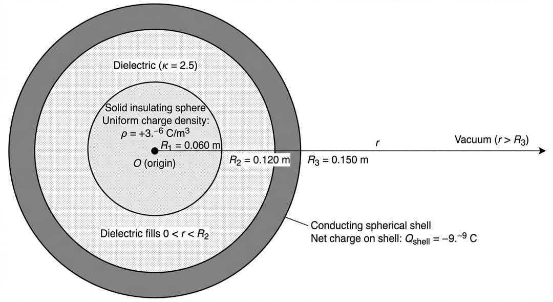
Figure 2. Bar chart template for the magnitude of the electric field |E| at specified radii, normalized to a reference bar at r = 0.200 m.

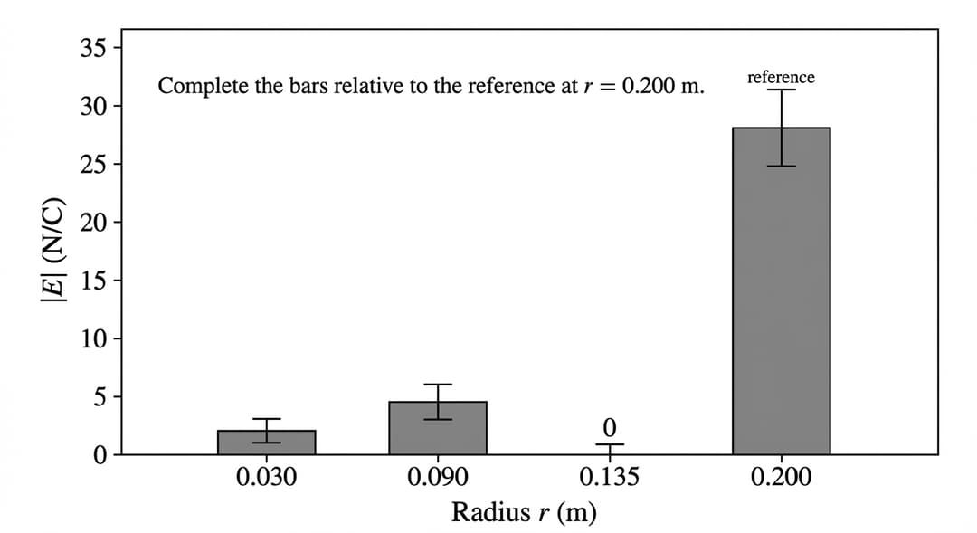
A single-panel bar chart with four categorical bars representing |E| at four radii.

Axes and frame:
- Horizontal axis label centered below the categories: "Radius r (m)".
- Four category tick labels (left to right), each centered under its bar:
1) "0.030"
2) "0.090"
3) "0.135"
4) "0.200"
- Vertical axis label rotated along the left side: "|E| (N/C)".
- Vertical axis numerical range: from 0 at the bottom to 35 at the top.
- Vertical axis tick marks and labels at every 5 N/C: "0, 5, 10, 15, 20, 25, 30, 35".
- The origin is shown at the bottom-left corner of the plot area with the y-axis labeled "0" at the baseline.
- Arrows: no arrows on either axis (standard bar-chart style).
- No gridlines.

Bar geometry and style:
- All four bars have identical width, each occupying a little over half of the spacing between category centers.
- Fill color: solid medium-gray.
- Outline: solid black outline with uniform medium stroke thickness.

Bar heights (EXACT numeric values):
- Bar at r = 0.030 m: height = 2.0 N/C.
- Bar at r = 0.090 m: height = 4.5 N/C.
- Bar at r = 0.135 m: height = 0.0 N/C (show as a visible "0" printed just above the baseline in this column, with no filled bar rising upward).
- Bar at r = 0.200 m (reference): height = 28.0 N/C.

Reference annotation:
- Above the r = 0.200 m bar, place a small text label: "reference".

Error bars (present on EVERY category, including the zero column):
- Each category has a vertical error bar drawn as a thin black line centered on the category, with horizontal caps at the top and bottom.
- Error-bar cap width: one-third of the bar width.
- Exact error-bar endpoints (not ± notation):
- r = 0.030 m bar: error bar from 1.6 to 2.4 N/C.
- r = 0.090 m bar: error bar from 3.9 to 5.1 N/C.
- r = 0.135 m column (mean 0.0): error bar from 0.0 to 0.8 N/C (bottom cap sits on the baseline at 0.0; top cap at 0.8).
- r = 0.200 m bar: error bar from 25.0 to 31.0 N/C.

Instructional text (small, above the plot but inside the figure border):
- "Complete the bars relative to the reference at r = 0.200 m."

In Figure 2, draw bars to represent $|E|$ at $r = 0.030\ \text{m}$ , $0.090\ \text{m}$ , and $0.135\ \text{m}$ relative to the $|E|$ shown at $r = 0.200\ \text{m}$ . If $|E| = 0$ , write a "0" in that column. Consider the magnitude of the electric field $|E|$ at four radial positions: $r = 0.030\ \text{m}$ , $0.090\ \text{m}$ , $0.135\ \text{m}$ , and $0.200\ \text{m}$ . The partially completed bar chart in Figure 2 shows a bar that represents $|E|$ at $r = 0.200\ \text{m}$ .

Derive an expression for the radial electric field $E_r(r)$ (including the correct sign for direction) in each of the following regions: (i) $0<r<R_1$ , (ii) $R_1<r<R_2$ , (iii) $R_2<r<R_3$ , and (iv) $r>R_3$ . Express your answers in terms of $\rho$ , $R_1$ , $R_2$ , $R_3$ , $Q_{\text{shell}}$ , $\kappa$ , $\varepsilon_0$ , and $r$ , as appropriate. Begin your derivation by writing a fundamental physics principle or an equation from the reference information.

Figure 3. Axes for sketching the radial electric field E_r versus radius r (outward positive).

A blank set of Cartesian-style axes intended for a hand-sketched curve of E_r versus r.

Axes:
- Horizontal axis: labeled "r (m)" centered below the axis.
- Horizontal axis range: from 0.000 m at the origin to 0.220 m at the right boundary.
- Horizontal tick marks and labels:
- Major ticks every 0.020 m, labeled "0.000, 0.020, 0.040, 0.060, 0.080, 0.100, 0.120, 0.140, 0.150, 0.160, 0.180, 0.200, 0.220".
- The three special radii are additionally emphasized with slightly longer tick marks and small labels directly above the axis: "R1", "R2", "R3" placed exactly at 0.060 m, 0.120 m, and 0.150 m respectively.

- Vertical axis: labeled "E_r (N/C)" along the left side.
- A direction note near the top of the vertical axis: "+ is outward".
- Vertical axis range: from −400 N/C at the bottom to +400 N/C at the top.
- Vertical axis tick marks and labels every 100 N/C: "−400, −300, −200, −100, 0, 100, 200, 300, 400".

Origin and arrows:
- The axes intersect at the lower-left corner of the plotting region, with the intersection explicitly labeled "0" on both axes.
- Arrows on the positive ends of both axes: rightward arrow on the r-axis and upward arrow on the E_r-axis.

Styling:
- Axes drawn with solid black lines, slightly thicker than tick marks.
- No gridlines, no plotted curve, and no legend.
- Only the axes, ticks, numeric labels, and the R1/R2/R3 markers are present.

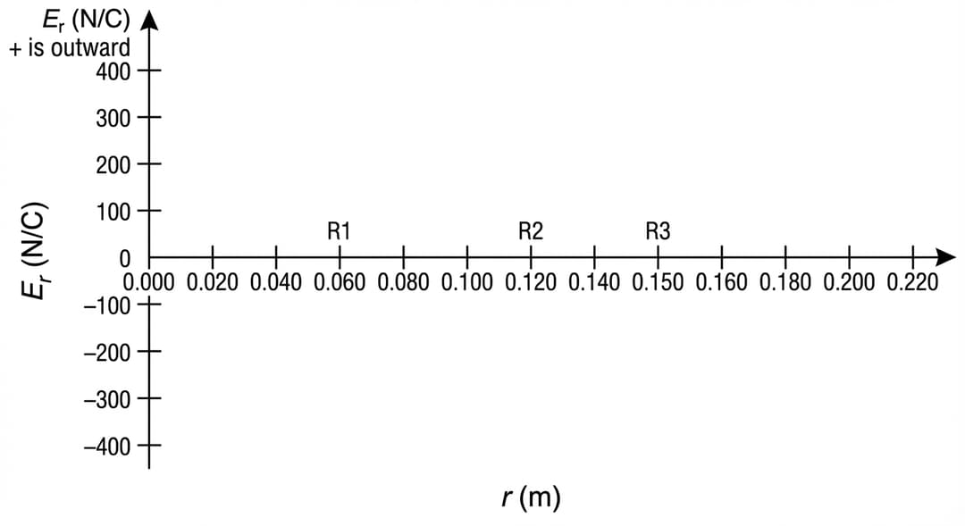
On the axes shown in Figure 3, sketch a graph of $E_r$ as a function of $r$ for $0<r<0.220\ \text{m}$ . Indicate any discontinuities or regions where $E_r=0$ .

Indicate whether the magnitude of the electric force on the particle at $r_0$ is greater than, less than, or equal to the magnitude of the gravitational force on the particle. Briefly justify your answer by calculating both force magnitudes at $r_0$ using your result from part B. A small particle of mass $m = 2.0\times10^{-6}\ \text{kg}$ and charge $q = -4.0\times10^{-9}\ \text{C}$ is released from rest at $r_0 = 0.090\ \text{m}$ . Assume the particle moves only radially and that gravitational interactions are due to Earth's gravitational field with $g = 9.8\ \text{m/s}^2$ directed in the $-\hat{y}$ direction. At the release point, the particle is located on the +y-axis (so outward radial direction is +y). Ignore any magnetic effects and any forces other than electric and gravitational forces. Use $\rho = +3.0\times10^{-6}\ \text{C/m}^3$ , $R_1 = 0.060\ \text{m}$ , $R_2 = 0.120\ \text{m}$ , $\kappa = 2.5$ , and $\varepsilon_0 = 8.85\times10^{-12}\ \text{C}^2/(\text{N}·\text{m}^2)$ .