Fiveable
🎡AP Physics 1
​

🎡AP Physics 1

FRQ 3 – Experimental Design
​
Unit 1: Kinematics
​
FRQ Types & Units

Each FRQ type tests specific skills taught in particular units. Here's why certain units appear for each question type:

This mapping reflects College Board's exam structure - each FRQ type tests specific skills that are taught in particular units.

Practice FRQ 1 of 151/15

3. Students are investigating the motion of objects as observed from different reference frames.

A.

Describe an experimental procedure to collect data that would allow the students to determine the velocity of Cart B relative to the track. Assume that Cart B moves with constant velocity in the positive direction along the track. Include any steps necessary to reduce experimental uncertainty. In your description, state what quantities would be measured and what equipment would be used to measure them.

B.

Describe how the data collected in part (A) could be graphed and how that graph would be analyzed to determine the velocity of Cart B relative to the track.

Figure 1. Two carts on a straight track

Black-and-white physics apparatus diagram (no perspective; clean textbook style) showing a single straight track with two carts and two motion sensors.

Overall layout:
- The track is drawn as two parallel horizontal rails forming a long, thin rectangle spanning nearly the full width of the figure.
- The track is centered vertically, with empty white space above and below for labels.
- A large arrow labeled "+x" is placed directly above the track near its center and points strictly to the right, indicating the positive direction along the track.

Cart placement (left-to-right order must be unambiguous):
- Cart A is positioned on the left half of the track, clearly left of the track’s midpoint.
- Cart B is positioned on the right half of the track, clearly right of the track’s midpoint.
- The horizontal gap between the two carts is large and visually obvious: the empty track space between them is wider than the length of either cart, so they are not close to touching.

Cart appearance (both carts consistent style):
- Each cart is a low rectangular body riding on the rails, with two visible wheels as solid circles.
- Each cart body has a bold label centered on the cart: the left cart labeled "Cart A" and the right cart labeled "Cart B".

Motion sensors (explicit orientation and placement):
- On Cart A: a small rectangular motion sensor is mounted on the RIGHT end (the front-facing end toward Cart B). The sensor’s "emitter/receiver" face is drawn as a dark vertical strip on its rightmost side.
- On Cart B: a small rectangular motion sensor is mounted on the LEFT end (the front-facing end toward Cart A). The sensor’s "emitter/receiver" face is drawn as a dark vertical strip on its leftmost side.
- Each sensor is labeled "motion sensor" with a short leader line pointing to the sensor body. The label for Cart A’s sensor sits above Cart A; the label for Cart B’s sensor sits above Cart B.

Direction arrows for cart motion (must match the written prompt):
- Near Cart B, include a single bold velocity arrow drawn just above Cart B, pointing strictly to the right and labeled "vB". This arrow communicates Cart B moves in the positive direction.
- Near Cart A, include a smaller double-headed arrow centered above Cart A (left-right arrowheads) labeled "Cart A can move" to indicate Cart A may move either direction during trials.

Track labeling:
- Centered below the track rails, place the label "track".

No numbers appear in this figure. No extra objects (no timers, photogates, or rulers) are shown. Only the track, two carts, two motion sensors, and the +x arrow are present.

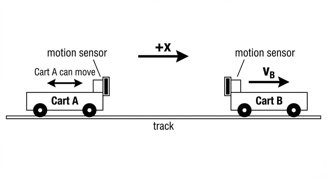
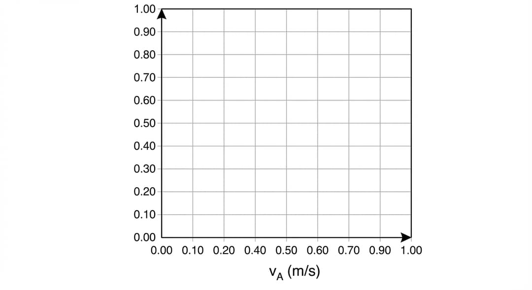
Figure 2. Grid for plotting a linearized graph

A square plotting grid designed for student graphing.

Grid frame and divisions:
- The grid is a square bounded by a dark outer border.
- Inside the border are evenly spaced light-gray gridlines forming exactly 10 equal major divisions across the width and exactly 10 equal major divisions up the height.
- The axes lie along the bottom edge (horizontal axis) and left edge (vertical axis), each drawn as a darker line than the interior gridlines.
- Each axis ends with a single arrowhead: the horizontal axis arrowhead points right; the vertical axis arrowhead points up.

Horizontal axis (pre-labeled; must include full numeric scale):
- Axis label centered below the horizontal axis: "vA (m/s)".
- The horizontal axis spans from 0.00 at the left end to 1.00 at the right end.
- Tick marks and tick labels appear at every 0.10 m/s: "0.00, 0.10, 0.20, 0.30, 0.40, 0.50, 0.60, 0.70, 0.80, 0.90, 1.00".
- The origin label "0.00" is placed at the bottom-left corner where the axes meet.

Vertical axis (intentionally blank label area but with numeric scale present for accurate plotting):
- The vertical axis has tick marks and tick labels but no variable name printed; a blank space is left to the left of the axis for students to write the vertical-axis quantity.
- The vertical axis spans from 0.00 at the bottom to 1.00 at the top.
- Tick marks and tick labels appear at every 0.10: "0.00, 0.10, 0.20, 0.30, 0.40, 0.50, 0.60, 0.70, 0.80, 0.90, 1.00".

Title and other text:
- No graph title is present.
- No legend is present.
- No data points are pre-plotted.

Styling constraints:
- All tick labels use the same font and are clearly legible.
- The interior gridlines are lighter than the axes and border so student points and best-fit lines stand out when added later.

vA (m/s)

vBA (m/s)

0.20

0.95

0.35

0.80

0.50

0.65

0.65

0.48

0.80

0.35

0.95

0.18

C.

The students perform an experiment in which Cart A is set to various constant velocities vA in the positive direction along the track. Cart B moves with constant velocity in the positive direction along the track. For each trial, the motion sensor on Cart A measures the velocity vBA of Cart B relative to Cart A. Table 1 shows the measured values of vA and vBA.

The students correctly determine that the relationship between vBA and vA is given by vBA = vB - vA, where vB is the velocity of Cart B relative to the track.

The students create a graph with vA plotted on the horizontal axis.

i.

Indicate what measured or calculated quantity could be plotted on the vertical axis to yield a linear graph whose slope can be used to calculate an experimental value for vB.

Vertical axis: Horizontal axis: vA

ii.

On the grid in Figure 2, plot the data points for the quantities indicated in part C(i). Use Table 2 to record any calculated quantities. Clearly label the vertical axis, including units as appropriate.

iii.

Draw a straight best-fit line for the data graphed in part C(ii).

D.

Using the best-fit line that you drew in part C(iii), calculate an experimental value for the velocity vB of Cart B relative to the track.


Pep

essential ap study content awaits..

Features
Testimonials
Testimonials
start studying →
FRQ Directions
Free Response Question Practice

This practice environment simulates the AP AP Physics 1 Free Response Questions section. Here are some guidelines:

  • Read each question carefullybefore responding. Pay attention to command verbs like "identify," "explain," "analyze," or "evaluate."
  • Use the timer to practice time management. You can pause, restart, or hide the timer as needed.
  • Mark for Review if you want to come back to a question later.
  • Your responses are saved automatically as you type. You can also use the drawing tool for questions that require diagrams or graphs.
  • Use the toolbar for formatting options like bold, italic, subscript, and superscript.
  • Navigate between questions using the Previous and Next buttons at the bottom of the screen.

Tip: Answer all parts of each question. Partial credit is often available, so even if you are unsure, provide what you know.