Multiple linear regression expands on simple linear regression by incorporating multiple predictors. This powerful statistical tool allows us to model complex relationships between variables, making it essential for data scientists and researchers analyzing real-world phenomena.

Understanding the components, evaluation methods, and challenges of multiple linear regression is crucial. This knowledge enables us to build accurate models, interpret results effectively, and address common issues like and in our analyses.

Model Components

Key Elements of Multiple Linear Regression

Top images from around the web for Key Elements of Multiple Linear Regression
  • represents the outcome or response being predicted
  • Independent variables serve as predictors or explanatory factors influencing the dependent variable
  • measure the change in the dependent variable for a one-unit increase in an , holding other variables constant
  • indicates the expected value of the dependent variable when all independent variables equal zero
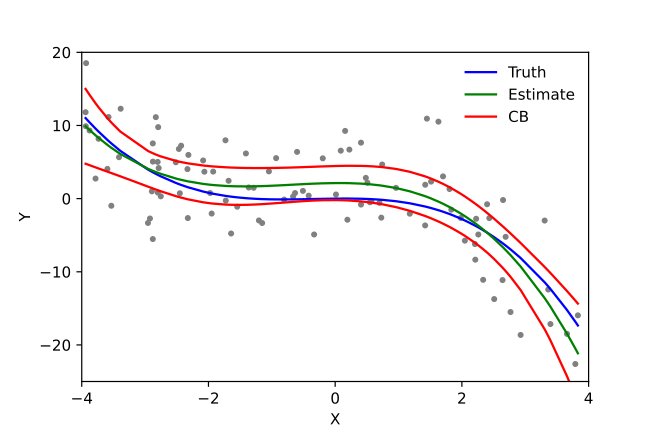
  • capture the difference between observed and predicted values, representing unexplained variation in the model

Mathematical Representation and Interpretation

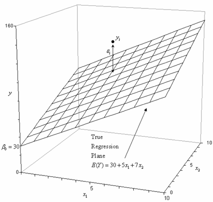
  • Multiple linear regression model expressed as: Y=β0+β1X1+β2X2+...+βkXk+εY = β₀ + β₁X₁ + β₂X₂ + ... + βₖXₖ + ε
  • Y denotes the dependent variable
  • X₁, X₂, ..., Xₖ represent k independent variables
  • β₀ symbolizes the intercept term
  • β₁, β₂, ..., βₖ correspond to regression coefficients for each independent variable
  • ε represents the error term or residuals
  • Interpretation of coefficients provides insights into the relative importance of each predictor variable

Model Evaluation

Estimation and Fitting Techniques

  • minimizes the sum of squared residuals to find optimal coefficient values
  • (OLS) method commonly used for parameter estimation in multiple linear regression
  • Calculation of least squares estimates involves matrix algebra and solving normal equations
  • measures assess how well the model explains the variation in the dependent variable

Performance Metrics and Interpretation

  • quantifies the proportion of variance in the dependent variable explained by the independent variables
  • R-squared ranges from 0 to 1, with higher values indicating better model fit
  • accounts for the number of predictors in the model, penalizing unnecessary complexity
  • Comparison between R-squared and adjusted R-squared helps identify potential overfitting issues
  • tests the overall significance of the regression model, comparing it to a null model

Model Challenges

Multicollinearity and Its Effects

  • Multicollinearity occurs when independent variables exhibit high correlation with each other
  • Consequences of multicollinearity include inflated standard errors and unstable coefficient estimates
  • Detection methods for multicollinearity involve correlation matrices and variance inflation factors
  • (VIF) quantifies the severity of multicollinearity for each predictor
  • VIF values greater than 5 or 10 typically indicate problematic levels of multicollinearity

Heteroscedasticity and Its Implications

  • Heteroscedasticity refers to non-constant variance of residuals across different levels of independent variables
  • Violates the assumption of homoscedasticity in multiple linear regression
  • Consequences of heteroscedasticity include biased standard errors and unreliable hypothesis tests
  • Detection methods for heteroscedasticity involve residual plots and statistical tests (Breusch-Pagan test)
  • Remedies for heteroscedasticity include weighted least squares regression and robust standard errors

Advanced Model Features

Incorporating Complex Relationships

  • capture the combined effect of two or more independent variables on the dependent variable
  • Multiplicative interaction modeled as: Y=β0+β1X1+β2X2+β3(X1X2)+εY = β₀ + β₁X₁ + β₂X₂ + β₃(X₁ * X₂) + ε
  • Interpretation of interaction terms requires considering the effect of one variable at different levels of another
  • Centering or standardizing variables helps mitigate multicollinearity issues in models with interaction terms

Handling Categorical Predictors

  • represent categorical variables with two or more levels in regression models
  • Creation of dummy variables involves assigning binary codes (0 or 1) to different categories
  • serves as the baseline for comparison in dummy variable coding
  • Interpretation of dummy variable coefficients compares each category to the reference category
  • extends dummy variable approach to categorical variables with multiple levels

Key Terms to Review (19)

Adjusted R-squared: Adjusted R-squared is a statistical measure that indicates the goodness of fit of a regression model while adjusting for the number of predictors in the model. Unlike R-squared, which can increase with the addition of more variables regardless of their relevance, adjusted R-squared provides a more accurate assessment by penalizing unnecessary complexity, ensuring that only meaningful predictors contribute to the overall model fit.
Dependent variable: A dependent variable is a key component in statistical modeling that represents the outcome or effect being studied, which is influenced by one or more independent variables. It is essentially what researchers measure to determine if changes in the independent variables lead to changes in this variable. In the context of regression analysis, the dependent variable is what you are trying to predict or explain based on other factors.
Dummy variables: Dummy variables are numerical variables used in regression analysis to represent categorical data. They allow for the inclusion of qualitative factors in a model by converting them into a series of binary variables, making it possible to capture the effects of these factors on the dependent variable. Dummy variables help in estimating relationships when the independent variables include non-numeric categories, enhancing the model's interpretability and validity.
F-statistic: The f-statistic is a ratio used to compare the variances of two or more groups in statistical models, particularly in the context of regression analysis and ANOVA. It helps determine whether the variance explained by the model is significantly greater than the unexplained variance, indicating that at least one group mean is different from the others. This concept is fundamental for assessing model performance and validating assumptions about the relationships among variables.
Goodness-of-fit: Goodness-of-fit refers to a statistical assessment that evaluates how well a model's predicted values align with the observed data. It's essential for determining the accuracy and reliability of statistical models, allowing researchers to judge whether the assumptions of the model are valid. A good goodness-of-fit indicates that the model adequately captures the underlying patterns in the data, which is crucial in both model diagnostics and multiple linear regression analyses.
Heteroscedasticity: Heteroscedasticity refers to the condition in regression analysis where the variance of the errors or residuals varies across different levels of an independent variable. This variability can lead to inefficient estimates and affect the validity of statistical tests, making it crucial to identify and address in model diagnostics, especially when validating multiple linear regression models and during diagnostic checks.
Homogeneity of Variance: Homogeneity of variance refers to the assumption that different samples or groups have the same variance or spread in their data. This concept is crucial for ensuring the reliability of statistical tests, as violations can lead to incorrect conclusions about relationships and differences in the data. In regression and analysis of variance contexts, it's particularly important for maintaining the validity of the results derived from models that rely on comparing group means or predicting outcomes based on multiple variables.
Independent Variable: An independent variable is a variable that is manipulated or controlled in an experiment to test its effects on the dependent variable. In statistical modeling, it serves as the predictor or explanatory factor, helping to understand how changes in this variable influence the outcome. Understanding independent variables is crucial for building predictive models and analyzing relationships between factors.
Interaction terms: Interaction terms are variables used in statistical models to assess how the effect of one predictor variable on the outcome variable changes depending on the level of another predictor variable. They help capture the combined effects of variables that may not be apparent when considering each predictor in isolation. Understanding interaction terms is crucial for developing accurate models that reflect complex relationships within data.
Intercept: In the context of multiple linear regression, the intercept is the expected value of the dependent variable when all independent variables are equal to zero. It represents the point where the regression line crosses the y-axis and is crucial for understanding how changes in the independent variables affect the dependent variable. The intercept provides a baseline from which predictions can be made, and it helps to interpret the overall model fit.
Least squares estimation: Least squares estimation is a statistical method used to determine the best-fitting line or hyperplane for a set of data points by minimizing the sum of the squares of the differences (residuals) between observed and predicted values. This technique is crucial in multiple linear regression as it provides a way to estimate the parameters that minimize prediction errors, ensuring that the model closely approximates the underlying data patterns.
Multicollinearity: Multicollinearity refers to the situation in which two or more independent variables in a regression model are highly correlated, meaning that they contain similar information about the variance in the dependent variable. This can lead to unreliable estimates of coefficients, inflated standard errors, and difficulty in determining the individual effect of each predictor. Understanding this concept is crucial when analyzing relationships between variables, evaluating model assumptions, and selecting appropriate variables for inclusion in regression models.
One-hot encoding: One-hot encoding is a technique used to convert categorical variables into a numerical format that can be used in machine learning models. This method creates binary columns for each category, where only one column is marked as '1' (hot) while the rest are marked as '0' (cold). This transformation is crucial for enabling algorithms to interpret categorical data without assuming any ordinal relationships.
Ordinary least squares: Ordinary least squares (OLS) is a statistical method used for estimating the parameters in a linear regression model by minimizing the sum of the squares of the differences between observed and predicted values. This technique aims to find the best-fitting line through the data points by determining the coefficients that result in the smallest possible error. OLS is fundamental in both simple and multiple regression analysis, as it provides a straightforward way to understand relationships between variables.
R-squared: R-squared is a statistical measure that represents the proportion of variance for a dependent variable that's explained by an independent variable or variables in a regression model. It indicates how well the data fits the model and helps assess the goodness-of-fit for both simple and multiple linear regression, guiding decisions about model adequacy and comparison.
Reference category: A reference category is a baseline group in categorical variables used in statistical models, particularly in regression analysis, to compare the effects of other categories. It serves as a point of reference against which the effects of the other categories are measured, enabling clearer interpretation of the results. This concept is essential for understanding how the different levels of categorical predictors influence the response variable in multiple linear regression models.
Regression coefficients: Regression coefficients are numerical values that represent the relationship between independent variables and the dependent variable in a regression model. They indicate how much the dependent variable is expected to change when one of the independent variables increases by one unit, while holding all other variables constant. Understanding these coefficients helps in interpreting the strength and direction of relationships within multiple linear regression models.
Residuals: Residuals are the differences between the observed values and the predicted values in a regression analysis. They help to assess how well a model fits the data, revealing whether the model captures the underlying patterns in the data or if there are systematic errors. Understanding residuals is crucial as they inform decisions on improving models and understanding variability in data.
Variance Inflation Factor: Variance inflation factor (VIF) is a measure used to detect multicollinearity in multiple regression models. It quantifies how much the variance of an estimated regression coefficient increases when your predictors are correlated. Understanding VIF is essential because high multicollinearity can inflate the standard errors of the coefficients, leading to unreliable statistical inferences and making it difficult to determine the effect of each predictor on the response variable.
© 2024 Fiveable Inc. All rights reserved.
AP® and SAT® are trademarks registered by the College Board, which is not affiliated with, and does not endorse this website.