Model validation and diagnostics are crucial for assessing the reliability of multiple linear regression models. These techniques help identify issues like , influential observations, and multicollinearity that can affect model performance and interpretation.

By examining , , and results, we can evaluate a model's predictive power and . This process ensures our regression models are robust and provide accurate insights for data-driven decision making.

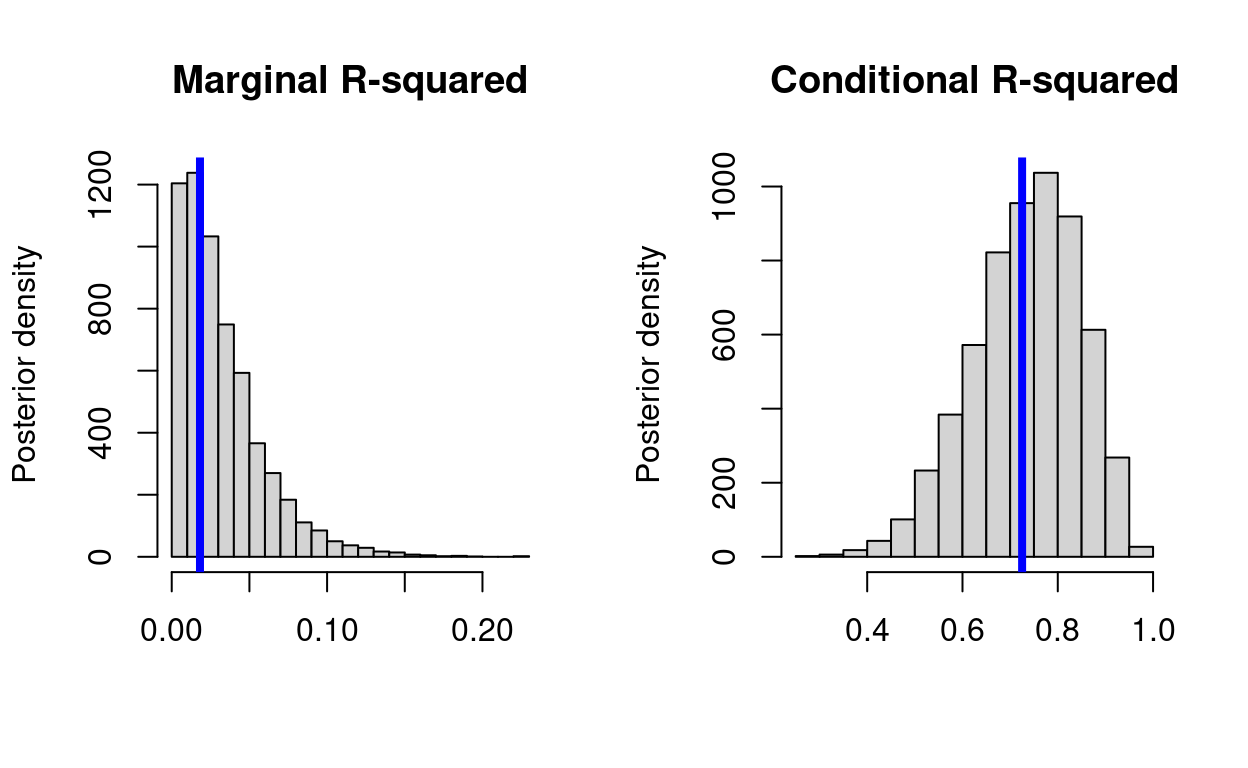
Goodness of Fit Measures

Coefficient of Determination and Adjusted Measure

Top images from around the web for Coefficient of Determination and Adjusted Measure
  • R-squared quantifies proportion of variance in dependent variable explained by independent variables
  • Ranges from 0 to 1, higher values indicate better fit
  • Calculated as ratio of explained variance to total variance: R2=1−SSESSTR^2 = 1 - \frac{SSE}{SST}
  • modifies R-squared to account for number of predictors
  • Penalizes addition of unnecessary variables to model
  • Formula incorporates degrees of freedom: Radj2=1−(1−R2)(n−1)n−k−1R^2_{adj} = 1 - \frac{(1-R^2)(n-1)}{n-k-1}
    • n represents number of observations
    • k denotes number of predictors

Statistical Significance and Prediction Error

  • assesses overall significance of regression model
  • Tests null hypothesis that all regression coefficients equal zero
  • Calculated as ratio of mean square regression to mean square error
  • Large F-statistic values suggest at least one predictor significantly related to response
  • PRESS (Prediction Error Sum of Squares) statistic measures model's predictive ability
  • Computed by summing squared prediction errors for each observation
  • Lower PRESS values indicate better predictive performance
  • Used in cross-validation to compare different models

Residual Diagnostics

Residual Analysis and Heteroscedasticity

  • examines differences between observed and predicted values
  • Helps identify violations of regression assumptions
  • Residuals calculated as ei=yi−y^ie_i = y_i - \hat{y}_i
  • Heteroscedasticity occurs when variance of residuals not constant across all predictor values
  • Detected through visual inspection of residual plots
  • Causes include:
    • Presence of outliers
    • Skewed distribution of dependent variable
    • Misspecification of model
  • Consequences of heteroscedasticity:
    • Inefficient parameter estimates
    • Biased standard errors
    • Invalid hypothesis tests and confidence intervals

Graphical Tools for Residual Assessment

  • assesses normality of residuals
  • Plots theoretical quantiles against sample quantiles
  • Straight line indicates normally distributed residuals
  • Residual plots visualize relationships between residuals and fitted values or predictors
  • Types of residual plots:
    • Residuals vs. Fitted values
    • Residuals vs. Predictors
    • Scale-Location plot
  • Patterns in residual plots suggest model inadequacies:
    • Funnel shape indicates heteroscedasticity
    • Curved pattern suggests non-linearity
    • Clustering suggests presence of subgroups in data

Influential Observations

Detecting Influential Points

  • measures influence of each observation on regression results
  • Quantifies change in regression coefficients when observation removed
  • Calculated for each data point: Di=(y^j−y^j(i))2p×MSE×hii(1−hii)2D_i = \frac{(\hat{y}_j - \hat{y}_{j(i)})^2}{p \times MSE} \times \frac{h_{ii}}{(1-h_{ii})^2}
  • Large Cook's distance values (typically > 4/n) indicate influential points
  • measures potential of observation to influence regression results
  • Determined by position of observation in predictor space
  • Calculated using hat matrix diagonal elements: hii=1n+(xi−xˉ)2∑j=1n(xj−xˉ)2h_{ii} = \frac{1}{n} + \frac{(x_i - \bar{x})^2}{\sum_{j=1}^n (x_j - \bar{x})^2}
  • High leverage points lie far from centroid of predictor space

Dealing with Influential Observations

  • Investigate reasons for influential observations:
    • Data entry errors
    • Unusual circumstances
    • Inherent variability in process
  • Options for handling influential points:
    • Remove if determined to be erroneous
    • Transform variables to reduce influence
    • Use robust regression techniques
  • Assess impact on model by comparing results with and without influential points
  • Document decisions and rationale for handling influential observations

Multicollinearity Assessment

Understanding and Detecting Multicollinearity

  • Multicollinearity occurs when strong correlations exist between predictor variables
  • Causes include:
    • Inherent relationships between variables
    • Redundant variables in model
    • Small sample sizes
  • Consequences of multicollinearity:
    • Inflated standard errors of coefficients
    • Unstable coefficient estimates
    • Difficulty interpreting individual predictor effects
  • Detection methods:
    • Correlation matrix analysis
    • Condition number of design matrix

Variance Inflation Factor (VIF)

  • VIF quantifies severity of multicollinearity for each predictor
  • Calculated as reciprocal of tolerance: VIFj=11−Rj2VIF_j = \frac{1}{1-R^2_j}
    • Rj2R^2_j when predictor j regressed on other predictors
  • Interpretation of VIF values:
    • VIF = 1: No correlation between predictor and other variables
    • 1 < VIF < 5: Moderate correlation
    • VIF > 5 or 10: High correlation, problematic multicollinearity
  • Addressing multicollinearity:
    • Remove highly correlated predictors
    • Combine correlated predictors into composite variables
    • Use regularization techniques (Ridge regression, Lasso)

Model Validation Techniques

Cross-validation Methods

  • Cross-validation assesses model's predictive performance on unseen data
  • Helps detect and estimate generalization error
  • K-fold cross-validation:
    • Divides data into k equally sized subsets
    • Uses k-1 subsets for training, 1 for validation
    • Repeats process k times, each subset used once for validation
    • Averages performance metrics across k iterations
  • Leave-one-out cross-validation (LOOCV):
    • Special case of k-fold where k equals number of observations
    • Computationally intensive for large datasets
  • Stratified cross-validation:
    • Ensures proportional representation of classes in each fold
    • Useful for imbalanced datasets

Evaluating Model Performance

  • Performance metrics for regression models:
    • Mean Squared Error (MSE)
    • Root Mean Squared Error (RMSE)
    • Mean Absolute Error (MAE)
    • R-squared on test set
  • Comparing cross-validation results:
    • Average performance across folds
    • Variability of performance across folds
  • :
    • : , low variance
    • Overfitting: Low bias,
    • Optimal model balances bias and variance
  • Using cross-validation for model selection:
    • Compare different model architectures
    • Tune hyperparameters
    • Select optimal feature subset

Key Terms to Review (32)

Accuracy: Accuracy is the measure of how close a predicted value or classification is to the actual value or true outcome. It plays a critical role in evaluating the performance of models, as it indicates how well a model can predict or classify data points correctly. High accuracy means that a significant proportion of predictions are correct, which is essential for building reliable and effective models.
Adjusted R-squared: Adjusted R-squared is a statistical measure that indicates the goodness of fit of a regression model while adjusting for the number of predictors in the model. Unlike R-squared, which can increase with the addition of more variables regardless of their relevance, adjusted R-squared provides a more accurate assessment by penalizing unnecessary complexity, ensuring that only meaningful predictors contribute to the overall model fit.
AIC: AIC, or Akaike Information Criterion, is a statistical measure used to compare different models and help identify the best fit among them while penalizing for complexity. It balances the goodness of fit of the model with a penalty for the number of parameters, which helps to avoid overfitting. This makes AIC valuable in various contexts, like choosing variables, validating models, applying regularization techniques, and analyzing time series data with ARIMA models.
Bias-Variance Tradeoff: The bias-variance tradeoff is a fundamental concept in machine learning and statistics that describes the balance between two sources of error that affect model performance: bias, which refers to the error due to overly simplistic assumptions in the learning algorithm, and variance, which refers to the error due to excessive sensitivity to fluctuations in the training data. Understanding this tradeoff is crucial for building models that generalize well to unseen data while avoiding both underfitting and overfitting.
BIC: BIC, or Bayesian Information Criterion, is a statistical tool used for model selection that helps to identify the best model among a set of candidates by balancing goodness of fit with model complexity. It penalizes models for having more parameters, thus helping to prevent overfitting while also considering how well the model explains the data. BIC is particularly useful in contexts like variable selection and regularization techniques where multiple models are compared.
Bootstrapping: Bootstrapping is a resampling technique used to estimate the distribution of a statistic by repeatedly sampling with replacement from a dataset. This method allows for the creation of multiple simulated samples, which can help in assessing the variability and reliability of estimates derived from the original data. It connects deeply with concepts like model validation, understanding sampling distributions, constructing confidence intervals, and promoting reproducible research practices.
Chi-square test: A chi-square test is a statistical method used to determine whether there is a significant association between categorical variables. It compares the observed frequencies in each category to the expected frequencies if there were no association, helping to validate models and assess goodness-of-fit.
Coefficient of determination: The coefficient of determination, often denoted as $R^2$, is a statistical measure that explains how well the independent variable(s) in a regression model predict the dependent variable. It provides insight into the proportion of variance in the dependent variable that can be explained by the independent variable(s), ranging from 0 to 1. A higher $R^2$ value indicates a better fit of the model to the data, which is crucial for assessing the effectiveness of predictive models.
Confusion Matrix: A confusion matrix is a table used to evaluate the performance of a classification model by comparing the predicted classifications to the actual classifications. It helps in understanding how well a model performs across different classes by showing true positives, false positives, true negatives, and false negatives. This matrix is essential for assessing metrics like accuracy, precision, recall, and F1 score, giving insights into where a model is succeeding or failing.
Cook's Distance: Cook's Distance is a measure used in regression analysis to identify influential data points that can disproportionately affect the estimated coefficients of a model. It evaluates how much the predicted values would change if a specific observation were removed from the dataset, helping in the assessment of model diagnostics and assumptions as well as model validation. Understanding Cook's Distance allows statisticians to address outliers and leverage points that could distort the model's predictions.
Cross-validation: Cross-validation is a statistical technique used to assess how the results of a predictive model will generalize to an independent data set. It is particularly useful in situations where the goal is to prevent overfitting, ensuring that the model performs well not just on training data but also on unseen data, which is vital for accurate predictions and insights.
F-statistic: The f-statistic is a ratio used to compare the variances of two or more groups in statistical models, particularly in the context of regression analysis and ANOVA. It helps determine whether the variance explained by the model is significantly greater than the unexplained variance, indicating that at least one group mean is different from the others. This concept is fundamental for assessing model performance and validating assumptions about the relationships among variables.
Generalizability: Generalizability refers to the extent to which findings from a specific study can be applied to broader populations or different contexts. It plays a crucial role in determining how well the results of a model or analysis hold true outside of the data set used to create it, affecting how confidently we can make predictions or draw conclusions based on the data.
Goodness of fit measures: Goodness of fit measures are statistical tests and metrics used to determine how well a model's predicted values match the observed data. They help in assessing the validity of a model by indicating whether the model adequately describes the underlying data structure. Understanding these measures is crucial for model validation, as they provide insight into how accurately a model reflects reality and whether it can be used for making predictions.
Heteroscedasticity: Heteroscedasticity refers to the condition in regression analysis where the variance of the errors or residuals varies across different levels of an independent variable. This variability can lead to inefficient estimates and affect the validity of statistical tests, making it crucial to identify and address in model diagnostics, especially when validating multiple linear regression models and during diagnostic checks.
High Bias: High bias refers to the error introduced by approximating a real-world problem, which can lead to an oversimplified model that fails to capture the underlying trends in the data. This often results in systematic errors in predictions and can manifest as poor performance on both training and validation datasets. High bias can be a result of underfitting, where the model is too simple relative to the complexity of the data.
High variance: High variance refers to a situation where a statistical model's predictions fluctuate widely, indicating that the model is too complex and sensitive to the training data. This often leads to overfitting, where the model captures noise in the data rather than the underlying patterns. As a result, high variance affects the model's ability to generalize well to new, unseen data.
K-fold validation: k-fold validation is a statistical method used to assess the performance of a predictive model by dividing the dataset into k equally sized subsets, or folds. The model is trained on k-1 folds and validated on the remaining fold, and this process is repeated k times, with each fold being used as the validation set once. This technique helps to provide a more reliable estimate of model performance by minimizing the impact of random data partitioning.
Kolmogorov-Smirnov Test: The Kolmogorov-Smirnov test is a non-parametric statistical test used to compare a sample distribution with a reference probability distribution, or to compare two sample distributions. This test helps in assessing whether the samples come from the same distribution, making it a valuable tool for model validation and diagnostics in statistical analysis.
Leave-one-out validation: Leave-one-out validation is a technique in model validation where a single observation is removed from the dataset and the model is trained on the remaining data. This process is repeated for each observation in the dataset, providing a robust method for assessing the model's performance. It allows for the evaluation of how well the model generalizes to unseen data by using every available sample for testing at least once.
Leverage: In the context of model validation and diagnostics, leverage refers to a measure of how much influence a particular observation has on the overall fit of a statistical model. High leverage points can disproportionately affect the results of a regression analysis, potentially leading to misleading conclusions if not properly addressed. Identifying and understanding leverage points is crucial for ensuring the integrity of model assessments and the validity of predictions.
Model robustness: Model robustness refers to the ability of a statistical model to perform reliably under varying conditions and assumptions. A robust model remains accurate and effective even when faced with outliers, noise, or changes in the underlying data distribution. This quality is essential for ensuring that predictions and inferences drawn from the model are valid across different scenarios and datasets.
Normal q-q plot: A normal q-q plot is a graphical tool used to assess if a dataset follows a normal distribution by plotting the quantiles of the data against the quantiles of a standard normal distribution. If the points on the plot fall approximately along a straight line, it suggests that the data is normally distributed, which is important for validating the assumptions of many statistical models.
Overfitting: Overfitting occurs when a statistical model captures noise or random fluctuations in the training data instead of the underlying data distribution, leading to poor generalization on new, unseen data. This happens when a model is too complex relative to the amount and noisiness of the data, resulting in high accuracy on training data but significantly lower accuracy on validation or test datasets.
Precision: Precision refers to the degree of consistency and reproducibility of measurements or predictions. In the context of model evaluation, precision is a measure of how many true positive results occur in comparison to the total number of positive predictions made by a model. It connects to the overall accuracy and reliability of models, ensuring that they yield trustworthy results when making predictions or classifications.
Prediction Error Sum of Squares (PRESS): Prediction Error Sum of Squares (PRESS) is a measure used to assess the predictive accuracy of a statistical model. It quantifies the discrepancy between the observed values and the predicted values generated by the model, specifically using data that was not included in the model fitting process. This metric is crucial for validating the model's performance and understanding how well it can generalize to new data.
Recall: Recall is a metric used to evaluate the performance of a model, particularly in classification tasks, reflecting the ability of the model to identify all relevant instances in a dataset. It focuses on the true positives identified by the model against the total actual positives, providing insight into how well the model captures important data points. High recall is crucial when the cost of missing positive instances is significant, making it a key factor in both model validation and selection processes.
Residual Analysis: Residual analysis involves examining the residuals, which are the differences between observed values and predicted values from a statistical model. This analysis helps assess the goodness of fit of the model, verify underlying assumptions, and detect patterns that may indicate issues like non-linearity or heteroscedasticity. By analyzing residuals, one can improve model performance and ensure the validity of inferences drawn from the model.
Residual Plots: Residual plots are graphical representations that show the residuals on the vertical axis against the fitted values or another variable on the horizontal axis. They are essential for diagnosing the appropriateness of a statistical model by revealing patterns that indicate potential issues such as non-linearity, heteroscedasticity, or outliers. Analyzing these plots helps in validating models and ensuring that assumptions underlying regression analyses are satisfied.
ROC Curve: The ROC (Receiver Operating Characteristic) Curve is a graphical representation used to evaluate the performance of a binary classification model by plotting the true positive rate against the false positive rate at various threshold settings. It is essential for understanding the trade-offs between sensitivity and specificity when selecting a model and helps in determining the optimal cutoff point for classification. The area under the ROC curve (AUC) quantifies the overall ability of the model to discriminate between positive and negative classes.
Underfitting: Underfitting occurs when a statistical model is too simple to capture the underlying patterns in the data, resulting in poor performance both on training and test datasets. This situation often leads to a model that fails to generalize well, as it cannot adequately represent the complexity of the data it is meant to learn from.
Variance Inflation Factor (VIF): Variance Inflation Factor (VIF) is a measure used to detect multicollinearity in regression analysis, quantifying how much the variance of a regression coefficient is increased due to linear relationships with other predictors. A high VIF indicates a high degree of multicollinearity, which can make the model estimates unreliable. Understanding VIF is crucial for model diagnostics and validating assumptions, as it helps in ensuring that the predictor variables do not excessively overlap in the information they provide.
© 2024 Fiveable Inc. All rights reserved.
AP® and SAT® are trademarks registered by the College Board, which is not affiliated with, and does not endorse this website.