Least squares estimation is a powerful method for finding the best-fitting line in . It minimizes the , providing optimal estimates for the and intercept of the regression equation.

This technique is crucial in simple linear regression, allowing us to quantify relationships between variables. By minimizing errors, least squares estimation helps create models that accurately predict outcomes and explain variability in data.

Linear Regression Model Components

Key Elements of Linear Regression

Top images from around the web for Key Elements of Linear Regression
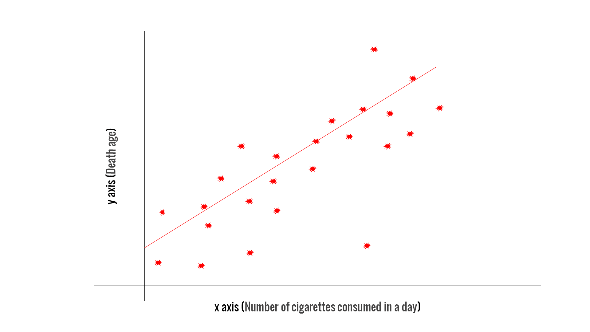
  • Linear regression model describes the relationship between two variables using a straight line
  • (Y) represents the outcome or response being predicted
  • (X) serves as the predictor or explanatory variable
  • Regression line forms the best-fit line through the data points
  • Slope (β1) measures the change in Y for a one-unit increase in X
  • (β0) indicates the of Y when X equals zero

Mathematical Representation

  • Linear regression equation: Y=β0+β1X+εY = β0 + β1X + ε
  • β0 and β1 are population parameters estimated from sample data
  • ε represents the error term, accounting for unexplained variation
  • Estimated regression equation: Y^=b0+b1XŶ = b0 + b1X
  • b0 and b1 are sample estimates of β0 and β1
  • Ŷ denotes the predicted value of Y for a given X

Interpreting Regression Components

  • indicates a direct relationship between X and Y
  • Negative slope signifies an inverse relationship between X and Y
  • Slope magnitude reflects the strength of the relationship
  • Y-intercept may have practical meaning in some contexts (initial value when X = 0)
  • Y-intercept can be meaningless or extrapolated beyond the data range in other cases

Residuals and Estimation

Understanding Residuals

  • measure the difference between observed and predicted Y values
  • Residual formula: ei=Yi−Y^ie_i = Y_i - Ŷ_i
  • Positive residuals indicate underestimation by the model
  • Negative residuals suggest overestimation by the model
  • Residual plot helps visualize model fit and detect patterns

Least Squares Estimation

  • Sum of squared residuals (SSR) quantifies the total squared deviation from the regression line
  • SSR formula: SSR=Σ(Yi−Y^i)2SSR = Σ(Y_i - Ŷ_i)^2
  • (OLS) method minimizes the SSR to find the best-fitting line
  • OLS estimates b0 and b1 to produce the smallest possible SSR
  • (BLUE) property ensures OLS estimates have minimum variance

Calculating Regression Coefficients

  • Slope estimate: b1=Σ(Xi−Xˉ)(Yi−Yˉ)Σ(Xi−Xˉ)2b1 = \frac{Σ(X_i - \bar{X})(Y_i - \bar{Y})}{Σ(X_i - \bar{X})^2}
  • Y-intercept estimate: b0=Yˉ−b1Xˉb0 = \bar{Y} - b1\bar{X}
  • \bar{X} and \bar{Y} represent the means of X and Y, respectively
  • These formulas provide point estimates for the regression

Model Evaluation Metrics

Assessing Model Fit

  • () measures the proportion of variance explained by the model
  • R-squared formula: R2=1−SSRSSTR^2 = 1 - \frac{SSR}{SST}
  • SST represents the total sum of squares: SST=Σ(Yi−Yˉ)2SST = Σ(Y_i - \bar{Y})^2
  • R-squared ranges from 0 to 1, with higher values indicating better fit
  • (SEE) quantifies the average deviation of observed Y values from the regression line
  • SEE formula: SEE=SSRn−2SEE = \sqrt{\frac{SSR}{n-2}}

Confidence and Prediction Intervals

  • provides a range for individual Y values at a given X
  • Prediction interval accounts for both model uncertainty and individual variation
  • estimates the range for the mean Y value at a given X
  • Confidence interval reflects only model uncertainty, not individual variation
  • Both intervals widen as X moves away from \bar{X}, indicating increased uncertainty

Interpreting Model Performance

  • Low R-squared suggests weak explanatory power of the independent variable
  • High R-squared indicates strong relationship between X and Y
  • Small SEE implies more precise predictions
  • Large SEE suggests less accurate predictions
  • Narrow confidence and prediction intervals indicate more reliable estimates
  • Wide intervals suggest less precise estimates and potential need for model improvement

Key Terms to Review (22)

Adjusted R-squared: Adjusted R-squared is a statistical measure that indicates the goodness of fit of a regression model while adjusting for the number of predictors in the model. Unlike R-squared, which can increase with the addition of more variables regardless of their relevance, adjusted R-squared provides a more accurate assessment by penalizing unnecessary complexity, ensuring that only meaningful predictors contribute to the overall model fit.
Best Linear Unbiased Estimator: The Best Linear Unbiased Estimator (BLUE) is a statistical estimator that provides the most accurate linear estimates of the parameters in a linear regression model, ensuring that these estimates are unbiased and have the smallest possible variance among all linear estimators. It combines properties of linearity, unbiasedness, and efficiency, making it an essential concept in least squares estimation. The Gauss-Markov theorem guarantees that under certain assumptions, the ordinary least squares (OLS) estimator is the BLUE.
Coefficient of determination: The coefficient of determination, often denoted as $R^2$, is a statistical measure that explains how well the independent variable(s) in a regression model predict the dependent variable. It provides insight into the proportion of variance in the dependent variable that can be explained by the independent variable(s), ranging from 0 to 1. A higher $R^2$ value indicates a better fit of the model to the data, which is crucial for assessing the effectiveness of predictive models.
Coefficients: Coefficients are numerical values that represent the strength and direction of the relationship between independent variables and a dependent variable in statistical models, particularly in regression analysis. They are crucial for interpreting how changes in the predictor variables impact the response variable, indicating the expected change in the dependent variable for a one-unit increase in the predictor, while holding other variables constant.
Confidence Interval: A confidence interval is a range of values that is used to estimate the true value of a population parameter, based on sample data. It provides an interval estimate with a specified level of confidence, indicating how sure we are that the parameter lies within that range. This concept is essential for understanding statistical inference, allowing for assessments of uncertainty and variability in data analysis.
Dependent variable: A dependent variable is a key component in statistical modeling that represents the outcome or effect being studied, which is influenced by one or more independent variables. It is essentially what researchers measure to determine if changes in the independent variables lead to changes in this variable. In the context of regression analysis, the dependent variable is what you are trying to predict or explain based on other factors.
Homoscedasticity: Homoscedasticity refers to the condition in which the variance of the errors in a regression model is constant across all levels of the independent variable(s). This property is crucial for valid hypothesis testing and reliable estimates in regression analysis. When homoscedasticity holds, it ensures that the model's predictions are equally reliable regardless of the value of the independent variable, which is vital for making sound inferences and decisions based on the data.
Independent Variable: An independent variable is a variable that is manipulated or controlled in an experiment to test its effects on the dependent variable. In statistical modeling, it serves as the predictor or explanatory factor, helping to understand how changes in this variable influence the outcome. Understanding independent variables is crucial for building predictive models and analyzing relationships between factors.
Linear regression: Linear regression is a statistical method used to model the relationship between a dependent variable and one or more independent variables by fitting a linear equation to observed data. This technique helps in understanding how the value of the dependent variable changes with variations in the independent variables, making it crucial for predictive analysis and data interpretation.
Linearity: Linearity refers to the relationship between two variables where a change in one variable results in a proportional change in another, often represented by a straight line on a graph. This concept is essential in various statistical methods, allowing for simplified modeling and predictions by assuming that relationships can be expressed as linear equations. In regression analysis, linearity is critical for understanding how well the model fits the data and provides insight into the strength and direction of relationships.
Mean Squared Error: Mean squared error (MSE) is a measure used to evaluate the accuracy of a predictive model by calculating the average squared difference between the estimated values and the actual values. It serves as a crucial metric for understanding how well a model performs, guiding decisions on model selection and refinement. By assessing the errors made by predictions, MSE helps highlight the balance between bias and variance, as well as the effectiveness of techniques like regularization and variable selection.
Ordinary least squares: Ordinary least squares (OLS) is a statistical method used for estimating the parameters in a linear regression model by minimizing the sum of the squares of the differences between observed and predicted values. This technique aims to find the best-fitting line through the data points by determining the coefficients that result in the smallest possible error. OLS is fundamental in both simple and multiple regression analysis, as it provides a straightforward way to understand relationships between variables.
Positive slope: A positive slope indicates that as the independent variable increases, the dependent variable also increases. This relationship is visually represented on a graph as an upward tilt from left to right. Positive slopes are essential in regression analysis, especially in least squares estimation, as they indicate a direct correlation between variables.
Predicted value: A predicted value is the estimated outcome or response of a dependent variable based on a statistical model and its independent variables. This value is derived from a regression equation, which helps in making forecasts or predictions about future observations based on existing data. The accuracy of predicted values relies heavily on the quality of the model and the underlying assumptions made during analysis.
Prediction Interval: A prediction interval is a range of values that is likely to contain the value of a new observation based on a statistical model, providing an estimate of uncertainty around the predicted outcome. This concept plays a crucial role in assessing how well a model can predict future data points and considers both the variability of the response variable and the uncertainty associated with estimating the parameters of the model.
R-squared: R-squared is a statistical measure that represents the proportion of variance for a dependent variable that's explained by an independent variable or variables in a regression model. It indicates how well the data fits the model and helps assess the goodness-of-fit for both simple and multiple linear regression, guiding decisions about model adequacy and comparison.
Residuals: Residuals are the differences between the observed values and the predicted values in a regression analysis. They help to assess how well a model fits the data, revealing whether the model captures the underlying patterns in the data or if there are systematic errors. Understanding residuals is crucial as they inform decisions on improving models and understanding variability in data.
Root Mean Squared Error: Root Mean Squared Error (RMSE) is a widely used metric for measuring the differences between predicted values and observed values in statistical modeling. It provides a way to quantify how well a model's predictions match actual outcomes, with lower RMSE values indicating better model performance. This concept is crucial in evaluating the accuracy of models, particularly in the context of regression analysis and model selection processes.
Slope: The slope in the context of a linear regression model represents the change in the dependent variable for each unit change in the independent variable. It essentially tells us how steep the line is and the direction of the relationship between the two variables, whether positive or negative. A positive slope indicates that as the independent variable increases, the dependent variable also increases, while a negative slope suggests an inverse relationship.
Standard Error of Estimate: The standard error of estimate measures the accuracy of predictions made by a regression model, indicating how much the observed values deviate from the predicted values. It helps in assessing the reliability of a linear regression model, giving insight into how well the model fits the data by quantifying the average distance that the observed values fall from the regression line. A smaller standard error of estimate suggests a better fit, as it indicates that the predicted values are closer to the actual values.
Sum of squared residuals: The sum of squared residuals is a statistical measure used to quantify the discrepancy between observed values and the values predicted by a regression model. It is calculated by taking the difference between each observed value and its corresponding predicted value, squaring these differences, and then summing them up. This measure is crucial in assessing the fit of a model, as smaller values indicate a better fit to the data.
Y-intercept: The y-intercept is the point where a line or curve crosses the y-axis on a graph, representing the value of the dependent variable when the independent variable is zero. In regression analysis, the y-intercept is crucial as it indicates the predicted value of the outcome variable when all predictor variables are set to zero, offering insight into the baseline level of the response. Understanding the y-intercept helps in interpreting the relationship between variables and assessing model fit.
© 2024 Fiveable Inc. All rights reserved.
AP® and SAT® are trademarks registered by the College Board, which is not affiliated with, and does not endorse this website.