Strong and are crucial concepts in parallel computing, measuring how well programs perform as resources increase. focuses on speeding up fixed-size problems, while weak scaling maintains as both workload and resources grow.

These scaling approaches help optimize parallel algorithms and systems, balancing factors like and . Understanding their nuances is key to designing scalable software and predicting performance in large-scale computing environments.

Strong vs Weak Scaling

Defining Strong and Weak Scaling

Top images from around the web for Defining Strong and Weak Scaling
  • Strong scaling measures achieved when increasing processor count for a fixed problem size
    • Aims to reduce execution time
    • Calculated as speedup divided by number of processors
  • Weak scaling evaluates execution time changes as problem size and processor count increase proportionally
    • Maintains constant workload per processor
    • Calculated as ratio of execution times between scaled and baseline cases
  • Ideal strong scaling results in linear speedup (doubling processors halves execution time)
  • Perfect weak scaling maintains constant execution time as both problem size and processor count increase

Theoretical Foundations

  • underpins strong scaling
    • Describes theoretical maximum speedup achievable for a given parallel fraction of the program
    • Formula: S(n)=1(1p)+pnS(n) = \frac{1}{(1-p) + \frac{p}{n}}
      • Where S is speedup, n is number of processors, p is parallel fraction
  • complements Amdahl's Law for weak scaling
    • Considers potential for problem size expansion with increased computational resources
    • Formula: S(n)=nα(n1)S(n) = n - \alpha(n - 1)
      • Where S is speedup, n is number of processors, α is serial fraction

Scalability of Parallel Algorithms

Scaling Analysis Techniques

  • Strong scaling analysis measures execution times for fixed problem size across varying processor counts
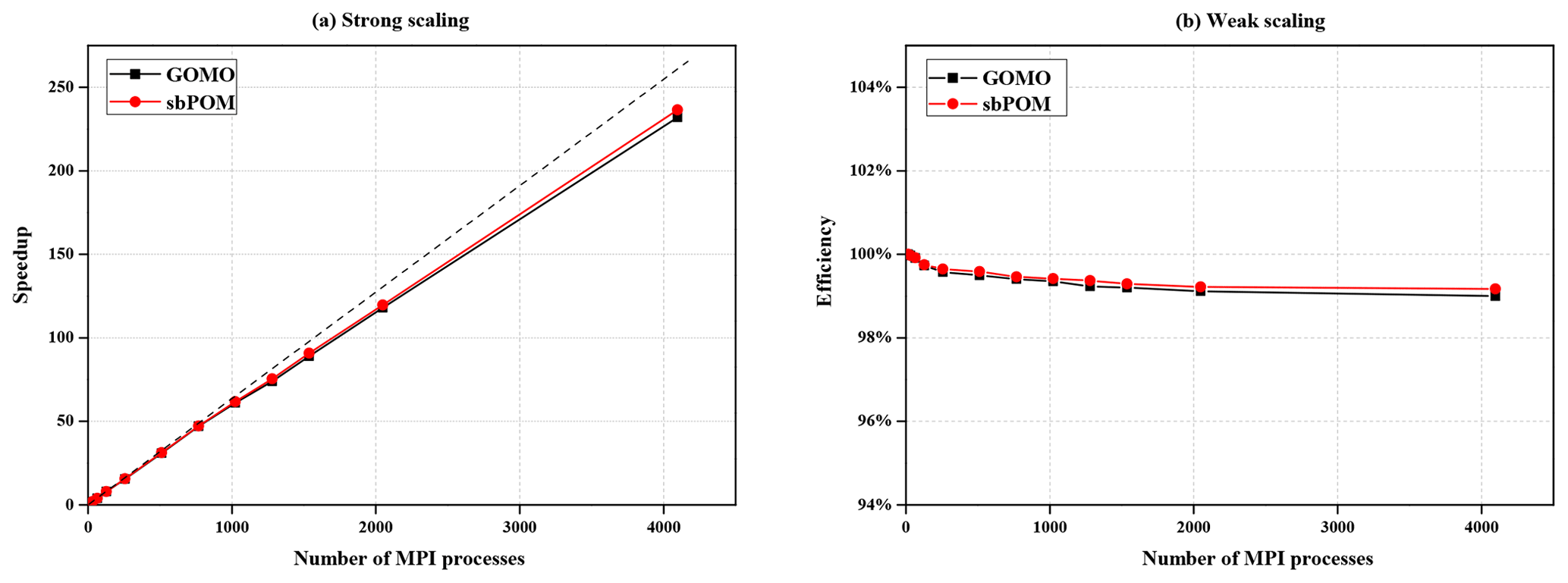
    • Typically plotted as speedup versus processor count
    • Example: Running a climate model simulation with fixed resolution on 1, 2, 4, 8, 16 processors
  • Weak scaling analysis adjusts problem size proportionally to processor count
    • Compares execution times to baseline single-processor run
    • Example: Increasing the number of particles in a molecular dynamics simulation proportionally to processor count
  • Isoefficiency analysis combines strong and weak scaling concepts
    • Determines how problem size must increase with processor count to maintain constant efficiency
    • Formula: W(p)=KT0(W(p),p)W(p) = K \cdot T_0(W(p), p)
      • Where W is problem size, p is number of processors, K is isoefficiency constant, T_0 is overhead function

Visualization and Metrics

  • Log-log plots of execution time versus problem size or processor count reveal scaling limits
    • Identify regions of diminishing returns
    • Example: Log-log plot showing execution time flattening as processor count increases beyond a certain point
  • Strong scaling efficiency quantifies algorithm's utilization of additional processors
    • Values closer to 1 (or 100%) indicate better scalability
    • Formula: Es=T1nTnE_s = \frac{T_1}{n \cdot T_n}
      • Where E_s is strong scaling efficiency, T_1 is execution time on 1 processor, n is number of processors, T_n is execution time on n processors
  • Weak scaling efficiency calculated by comparing execution times of scaled runs to baseline
    • Consistent times across scales indicate good weak scalability
    • Formula: Ew=T1TnE_w = \frac{T_1}{T_n}
      • Where E_w is weak scaling efficiency, T_1 is execution time on 1 processor, T_n is execution time on n processors with n times larger problem

Factors Affecting Scaling Performance

Problem and Algorithm Characteristics

  • Problem size significantly impacts strong scaling
    • Larger problems generally exhibit better strong scaling due to improved computation-to-communication ratios
    • Example: Matrix multiplication scaling better for 10000x10000 matrices compared to 100x100 matrices
  • Algorithmic characteristics determine scaling potential
    • Degree of inherent parallelism affects maximum achievable speedup
    • Task dependencies limit parallelization opportunities
    • Example: Embarrassingly parallel algorithms (Monte Carlo simulations) scale better than algorithms with complex dependencies (Gauss-Seidel iteration)
  • Communication-to-computation ratio often determines practical parallelization limits
    • High ratios lead to diminishing returns in strong scaling
    • Example: N-body simulations becoming communication-bound at high processor counts

System and Implementation Factors

  • Load balancing crucial for both strong and weak scaling
    • Imbalanced workloads lead to processor idling and reduced efficiency
    • Example: Uneven particle distribution in spatial decomposition of molecular dynamics simulations
  • Communication overhead (latency, bandwidth limitations) often limits strong scaling at high processor counts
    • Example: All-to-all communication patterns in FFT algorithms becoming bottlenecks
  • Memory hierarchy and cache effects impact both scaling types
    • Changes in data distribution across processors alter cache utilization
    • Example: Cache-oblivious algorithms maintaining performance across different problem sizes and processor counts
  • System architecture influences scaling behavior
    • Interconnect topology affects communication patterns
    • Memory organization impacts data access times
    • Example: Torus interconnects providing better scaling for nearest-neighbor communication patterns compared to bus-based systems
  • I/O operations can become bottlenecks in both scaling scenarios
    • Particularly impactful for data-intensive applications
    • Example: Parallel file systems (Lustre, GPFS) improving I/O scalability in large-scale simulations

Evaluating Parallel System Efficiency

Performance Curves and Metrics

  • Speedup curves plot relative performance improvement against processor count
    • Shape indicates degree of scalability
    • Example: Linear speedup curve for embarrassingly parallel problems vs. sublinear curve for communication-bound algorithms
  • Efficiency curves demonstrate utilization of additional resources
    • Declining curves suggest diminishing returns in scalability
    • Formula: E(n)=S(n)nE(n) = \frac{S(n)}{n}
      • Where E is efficiency, S is speedup, n is number of processors
  • Iso-efficiency functions determine problem size increase rate to maintain efficiency
    • Help identify scalability limits
    • Example: Iso-efficiency function for matrix multiplication: W=Ω(p3/2)W = \Omega(p^{3/2})
      • Where W is problem size, p is number of processors
  • Scalability vectors combine multiple metrics for comprehensive performance view
    • Include factors like speedup, efficiency, and problem size scaling
    • Example: 3D vector (speedup, efficiency, communication overhead) tracking scaling behavior

Advanced Analysis Techniques

  • Crossover points in scaling curves identify transitions between scaling regimes
    • Example: Transition from computation-bound to communication-bound behavior in strong scaling of iterative solvers
  • Roofline models adapted for scaling analysis
    • Incorporate communication costs and parallel efficiency into performance bounds
    • Example: Extended roofline model showing how communication bandwidth limits achievable performance at high processor counts
  • Scalability prediction models estimate large-scale performance
    • Based on analytical or empirical approaches
    • Example: LogGP model predicting communication overhead for different system sizes
  • Gustafson-Barsis' Law used for weak scaling predictions
    • Estimates speedup for scaled problem sizes
    • Formula: S=pα(p1)S = p - \alpha(p - 1)
      • Where S is speedup, p is number of processors, α is serial fraction

Key Terms to Review (16)

Amdahl's Law: Amdahl's Law is a formula that helps to find the maximum improvement of a system's performance when only part of the system is improved. This concept is crucial in parallel computing, as it illustrates the diminishing returns of adding more processors or resources when a portion of a task remains sequential. Understanding Amdahl's Law allows for better insights into the limits of parallelism and guides the optimization of both software and hardware systems.
Benchmarking: Benchmarking is the process of measuring the performance of a system, application, or algorithm against a standard or set of criteria, often to assess efficiency and effectiveness. This practice helps identify areas for improvement and optimization, making it essential for analyzing parallel programs, understanding scaling behavior, and evaluating performance metrics. By establishing benchmarks, developers can make informed decisions about where to allocate resources and how to enhance system performance.
Communication overhead: Communication overhead refers to the time and resources required for data exchange among processes in a parallel or distributed computing environment. It is crucial to understand how this overhead impacts performance, as it can significantly affect the efficiency and speed of parallel applications, influencing factors like scalability and load balancing.
Distributed memory systems: Distributed memory systems are a type of computer architecture where each processor has its own private memory. In this setup, processors communicate and share data by passing messages rather than accessing a shared memory space. This architecture is essential in parallel computing, as it allows for scalability and efficient resource utilization when handling large computations.
Efficiency: Efficiency in computing refers to the ability of a system to maximize its output while minimizing resource usage, such as time, memory, or energy. In parallel and distributed computing, achieving high efficiency is crucial for optimizing performance and resource utilization across various models and applications.
Gustafson's Law: Gustafson's Law is a principle in parallel computing that argues that the speedup of a program is not limited by the fraction of code that can be parallelized but rather by the overall problem size that can be scaled with more processors. This law highlights the potential for performance improvements when the problem size increases with added computational resources, emphasizing the advantages of parallel processing in real-world applications.
Load Balancing: Load balancing is the process of distributing workloads across multiple computing resources to optimize resource use, minimize response time, and avoid overload of any single resource. This technique is essential in maximizing performance in both parallel and distributed computing environments, ensuring that tasks are allocated efficiently among available processors or nodes.
Map-Reduce: Map-Reduce is a programming model designed for processing large data sets across distributed systems. It divides tasks into two main functions: 'map', which processes input data and produces key-value pairs, and 'reduce', which aggregates those pairs to produce a final output. This model is vital for efficient data processing in parallel computing, ensuring scalability and performance optimization.
MPI: MPI, or Message Passing Interface, is a standardized and portable message-passing system designed for parallel programming, which allows processes to communicate with one another in a distributed computing environment. It provides a framework for developing parallel applications by enabling data exchange between processes, regardless of whether they are on the same machine or across different nodes in a cluster. Its design addresses challenges in synchronization, performance, and efficient communication that arise in high-performance computing.
OpenMP: OpenMP is an API that supports multi-platform shared memory multiprocessing programming in C, C++, and Fortran. It provides a simple and flexible interface for developing parallel applications by enabling developers to specify parallel regions and work-sharing constructs, making it easier to utilize the capabilities of modern multicore processors.
Parallel sorting algorithms: Parallel sorting algorithms are methods used to sort large datasets by dividing the sorting task into smaller subtasks that can be executed simultaneously across multiple processors. This approach takes advantage of parallel processing to reduce the time complexity of sorting, making it particularly effective for large-scale data applications where performance is crucial. By optimizing how data is divided and merged, these algorithms play a vital role in achieving efficient computation and scalability.
Profiling: Profiling is the process of analyzing a program's behavior and performance to identify areas for improvement, specifically in terms of speed and resource usage. By examining how the program executes, which functions are time-consuming, and how memory is utilized, developers can optimize their code for better efficiency and scalability. Profiling is essential for understanding the performance characteristics of both parallel and distributed systems, allowing for effective optimization techniques and scalability analysis.
Shared memory systems: Shared memory systems are computing architectures that allow multiple processors to access a common memory space, facilitating communication and data exchange between them. This design is key in enabling efficient collaboration on tasks, where all processors can read from and write to the same memory area without needing explicit message passing. This approach has significant implications for both strong and weak scaling, as it directly influences how workloads are distributed and processed across multiple processors.
Speedup: Speedup is a performance metric that measures the improvement in execution time of a parallel algorithm compared to its sequential counterpart. It provides insights into how effectively a parallel system utilizes resources to reduce processing time, highlighting the advantages of using multiple processors or cores in computation.
Strong Scaling: Strong scaling refers to the ability of a parallel computing system to increase its performance by adding more processors while keeping the total problem size fixed. This concept is crucial for understanding how well a computational task can utilize additional resources without increasing the workload, thus impacting efficiency and performance across various computing scenarios.
Weak Scaling: Weak scaling refers to the ability of a parallel computing system to maintain constant performance levels as the problem size increases proportionally with the number of processors. This concept is essential in understanding how well a system can handle larger datasets or more complex computations without degrading performance as more resources are added.
© 2024 Fiveable Inc. All rights reserved.
AP® and SAT® are trademarks registered by the College Board, which is not affiliated with, and does not endorse this website.