Parallel algorithms need to be fast and efficient, but how do we measure that? Performance metrics and analysis help us understand how well our algorithms work as we throw more processors at them.

We'll look at key metrics like and , and explore how to measure them. We'll also dive into scalability, which tells us if our algorithm can handle bigger problems or more processors without breaking a sweat.

Key performance metrics for parallel algorithms

Fundamental metrics and ratios

Top images from around the web for Fundamental metrics and ratios
  • Execution time measures total computation duration including computation and communication time
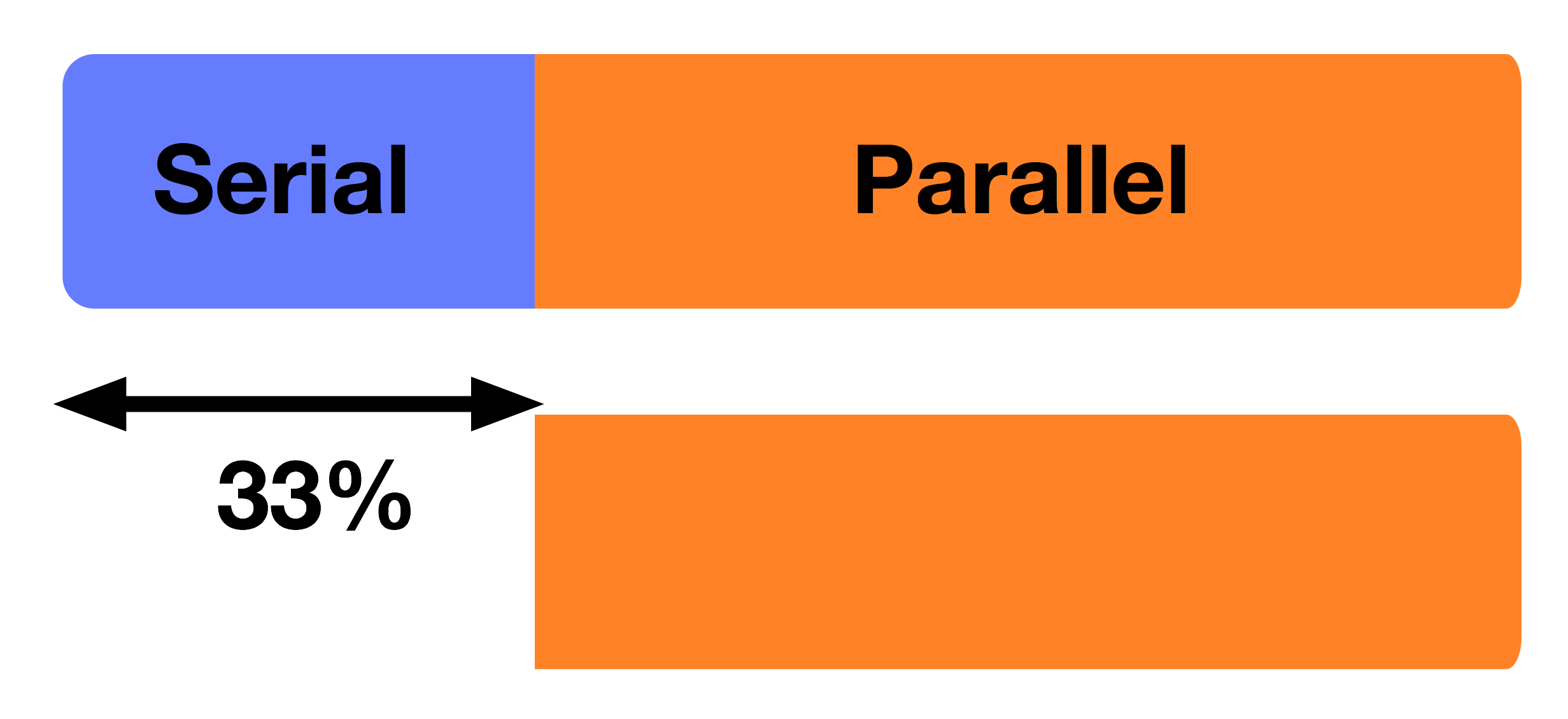
  • Speedup quantifies performance gain compared to sequential counterpart
    • Calculated as ratio of sequential execution time to parallel execution time
  • Efficiency evaluates effective resource utilization
    • Computed as ratio of speedup to number of processors used
  • defined as product of parallel runtime and number of processors
    • Provides insight into algorithm's resource utilization
  • quantifies additional inter-processor communication time
    • Can significantly impact parallel performance (network congestion, )

Scalability measures

  • Scalability assesses algorithm's ability to maintain performance as problem size or processor count increases
  • relates problem size to processors required for constant efficiency
    • Serves as measure of algorithm's scalability
    • Helps determine how quickly problem size must grow to maintain efficiency
  • examines speedup with fixed problem size and increasing processors
  • analyzes performance with fixed problem size per processor

Measuring speedup, efficiency, and scalability

Calculating key metrics

  • Speedup calculated by dividing sequential execution time by parallel execution time
    • Linear speedup ideal but rarely achievable (hardware limitations, overhead)
  • Efficiency computed as speedup divided by number of processors
    • Values range from 0 to 1, with 1 representing perfect efficiency
    • Efficiency of 0.8 indicates 80% utilization of available processing power
  • Scalability analysis involves plotting speedup or efficiency vs number of processors
    • Visualizes performance trends and identifies scaling limitations
    • Logarithmic scales often used for large processor counts

Theoretical models and laws

  • provides theoretical upper bound on speedup
    • Based on fraction of algorithm that can be parallelized
    • Highlights impact of sequential bottlenecks
    • Formula: S(n)=1(1p)+pnS(n) = \frac{1}{(1-p) + \frac{p}{n}} where p is parallelizable fraction, n is number of processors
  • offers alternative perspective on speedup
    • Focuses on tackling larger problems in same time as sequential systems
    • Formula: S(n)=nα(n1)S(n) = n - \alpha(n-1) where α is serial fraction of parallel execution time

Interpreting results

  • Consider factors affecting observed performance patterns:
    • Problem size (may reveal different scaling behavior for small vs large problems)
    • Algorithm structure (embarrassingly parallel vs tightly coupled)
    • Hardware characteristics (, network topology)
  • Identify scaling regimes:
    • (ideal case, speedup proportional to processors)
    • (common, diminishing returns as processors increase)
    • (rare, can occur due to cache effects)

Scalability of parallel algorithms

Theoretical analysis techniques

  • Derive mathematical models of algorithm performance based on structure and computational complexity
  • Apply asymptotic analysis (big O notation) to understand scalability as problem size approaches infinity
  • Utilize isoefficiency function to determine problem size growth rate for constant efficiency
    • Example: W=KPlog2PW = KP \log_2 P for many divide-and-conquer algorithms, where W is problem size, P is processors, K is constant
  • Employ performance modeling frameworks:
    • considers latency, overhead, gap, and processor count
    • BSP (Bulk Synchronous Parallel) model analyzes computation, communication, and synchronization phases

Empirical analysis methods

  • Conduct experiments on real parallel systems
    • Measure performance metrics for various problem sizes and processor counts
    • Use suites (PARSEC, NAS Parallel Benchmarks) for standardized analysis
  • Apply statistical methods to analyze results:
    • Regression analysis fits empirical data to theoretical models
    • Extrapolate scalability trends beyond measured data points
  • Visualize results using scaling plots:
    • Speedup vs processors (reveals deviation from ideal linear speedup)
    • Efficiency vs processors (shows how well system utilizes additional resources)
    • Execution time vs problem size (demonstrates weak scaling behavior)

Combining theoretical and empirical approaches

  • Validate theoretical models with empirical data
    • Identify discrepancies and refine models accordingly
  • Use theoretical insights to guide empirical experiments
    • Focus on predicted bottlenecks or interesting scaling regions
  • Iteratively improve understanding of algorithm scalability
    • Refine models based on experimental observations
    • Design new experiments to test theoretical predictions

Factors limiting scalability and optimizations

Workload distribution and communication

  • Load imbalance creates idle time and reduces scalability
    • Implement techniques (work stealing, task queues)
    • Example: In parallel matrix multiplication, use block cyclic distribution instead of simple block partitioning
  • Communication overhead increases with processor count
    • Minimize data transfers (local computations, data )
    • Use efficient communication patterns (collective operations, topology-aware algorithms)
    • Example: Reduce all-to-all communication in parallel FFT by using butterfly communication pattern

Algorithm structure and synchronization

  • Synchronization points create bottlenecks
    • Apply barrier elimination techniques
    • Develop asynchronous algorithms where possible
    • Example: Replace global barriers with point-to-point synchronization in parallel iterative solvers
  • Sequential portions limit overall scalability (Amdahl's Law)
    • Identify and parallelize sequential sections
    • Redesign algorithms with inherent parallelism
    • Example: Parallelize initialization and result collection phases in parallel simulations

Hardware constraints and optimizations

  • Memory limitations restrict scalability in shared memory systems
    • Implement data locality optimizations (cache blocking, data layout transformations)
    • Develop cache-aware and cache-oblivious algorithms
    • Example: Use cache-friendly Morton order for matrix traversals in parallel linear algebra routines
  • Network topology and interconnect bandwidth can limit scalability
    • Consider hardware characteristics in algorithm design (hierarchical algorithms for NUMA systems)
    • Optimize for specific network topologies (hypercube algorithms for fat-tree networks)
    • Example: Implement topology-aware MPI collective operations for improved performance on large-scale systems

Key Terms to Review (24)

Amdahl's Law: Amdahl's Law is a formula that helps to find the maximum improvement of a system's performance when only part of the system is improved. This concept is crucial in parallel computing, as it illustrates the diminishing returns of adding more processors or resources when a portion of a task remains sequential. Understanding Amdahl's Law allows for better insights into the limits of parallelism and guides the optimization of both software and hardware systems.
Bandwidth: Bandwidth refers to the maximum rate at which data can be transmitted over a communication channel or network in a given amount of time. It is a critical factor that influences the performance and efficiency of various computing architectures, impacting how quickly data can be shared between components, whether in shared or distributed memory systems, during message passing, or in parallel processing tasks.
Benchmarking: Benchmarking is the process of measuring the performance of a system, application, or algorithm against a standard or set of criteria, often to assess efficiency and effectiveness. This practice helps identify areas for improvement and optimization, making it essential for analyzing parallel programs, understanding scaling behavior, and evaluating performance metrics. By establishing benchmarks, developers can make informed decisions about where to allocate resources and how to enhance system performance.
Bulk Synchronous Parallel (BSP): Bulk Synchronous Parallel (BSP) is a parallel computing model that emphasizes a structure where computation is divided into a sequence of supersteps, each consisting of local computations followed by a global synchronization phase. This model allows for predictable performance and scalability, making it easier to analyze and understand the behavior of parallel algorithms as the number of processors increases.
Checkpointing: Checkpointing is a fault tolerance technique used in computing systems, particularly in parallel and distributed environments, to save the state of a system at specific intervals. This process allows the system to recover from failures by reverting back to the last saved state, minimizing data loss and reducing the time needed to recover from errors.
Communication overhead: Communication overhead refers to the time and resources required for data exchange among processes in a parallel or distributed computing environment. It is crucial to understand how this overhead impacts performance, as it can significantly affect the efficiency and speed of parallel applications, influencing factors like scalability and load balancing.
Cost: In the context of performance metrics and scalability analysis, cost refers to the resources consumed by a system to execute tasks, typically measured in terms of time, energy, or financial expense. Understanding cost is essential for evaluating the efficiency and effectiveness of computing systems, particularly as they scale. It helps identify bottlenecks and informs decisions on resource allocation, allowing for optimal performance as demands increase.
Dynamic load balancing: Dynamic load balancing is the process of distributing workloads across multiple computing resources in real-time, adapting to varying conditions and system loads to optimize performance. This approach is crucial in ensuring that no single resource becomes a bottleneck, especially in environments where tasks may have unpredictable execution times or where the number of tasks can change frequently. By continually monitoring and redistributing workloads, dynamic load balancing enhances efficiency and resource utilization.
Efficiency: Efficiency in computing refers to the ability of a system to maximize its output while minimizing resource usage, such as time, memory, or energy. In parallel and distributed computing, achieving high efficiency is crucial for optimizing performance and resource utilization across various models and applications.
Gustafson's Law: Gustafson's Law is a principle in parallel computing that argues that the speedup of a program is not limited by the fraction of code that can be parallelized but rather by the overall problem size that can be scaled with more processors. This law highlights the potential for performance improvements when the problem size increases with added computational resources, emphasizing the advantages of parallel processing in real-world applications.
Isoefficiency Function: The isoefficiency function is a performance metric that helps assess the scalability of parallel algorithms by measuring how the computational resources must increase to maintain efficiency as the problem size grows. It illustrates the relationship between the number of processors used and the size of the problem, providing insight into whether an algorithm can effectively utilize additional resources without diminishing returns. Understanding this function is crucial for evaluating and designing scalable parallel systems.
Latency: Latency is the time delay experienced in a system when transferring data from one point to another, often measured in milliseconds. It is a crucial factor in determining the performance and efficiency of computing systems, especially in parallel and distributed computing environments where communication between processes can significantly impact overall execution time.
Linear scaling: Linear scaling refers to the ability of a system to maintain consistent performance levels as resources are added, meaning that doubling the resources will double the performance. This concept is crucial in understanding how efficiently a system can handle increased workloads, which is directly linked to performance metrics and scalability analysis.
Logp model: The logp model is a theoretical framework used to analyze and evaluate the performance of parallel and distributed computing systems. It focuses on key parameters such as latency, overhead, granularity, and the number of processing units to better understand how these systems scale and perform under various conditions.
Memory Bandwidth: Memory bandwidth refers to the rate at which data can be read from or written to the memory by a processor, typically measured in bytes per second. It plays a crucial role in determining the performance of computing systems, especially in environments that rely on shared memory, as it affects how quickly processors can access data needed for processing. High memory bandwidth allows for better utilization of processing power, ultimately enhancing application performance and scalability.
Profiling: Profiling is the process of analyzing a program's behavior and performance to identify areas for improvement, specifically in terms of speed and resource usage. By examining how the program executes, which functions are time-consuming, and how memory is utilized, developers can optimize their code for better efficiency and scalability. Profiling is essential for understanding the performance characteristics of both parallel and distributed systems, allowing for effective optimization techniques and scalability analysis.
Replication: Replication refers to the process of creating copies of data or computational tasks to enhance reliability, performance, and availability in distributed and parallel computing environments. It is crucial for fault tolerance, as it ensures that even if one copy fails, others can still provide the necessary data or services. This concept is interconnected with various system architectures and optimization techniques, highlighting the importance of maintaining data integrity and minimizing communication overhead.
Scalability: Scalability refers to the ability of a system, network, or process to handle a growing amount of work or its potential to be enlarged to accommodate that growth. It is crucial for ensuring that performance remains stable as demand increases, making it a key factor in the design and implementation of parallel and distributed computing systems.
Speedup: Speedup is a performance metric that measures the improvement in execution time of a parallel algorithm compared to its sequential counterpart. It provides insights into how effectively a parallel system utilizes resources to reduce processing time, highlighting the advantages of using multiple processors or cores in computation.
Static Load Balancing: Static load balancing is a technique used in parallel computing where the distribution of tasks to various processors is determined before the execution begins, ensuring that each processor receives a predetermined workload. This approach does not adapt to runtime conditions and relies on the knowledge of task characteristics and processing capabilities, making it essential for maintaining performance in distributed systems. The efficiency of static load balancing can significantly influence performance metrics, especially when considering scalability and optimization strategies in heterogeneous environments.
Strong Scaling: Strong scaling refers to the ability of a parallel computing system to increase its performance by adding more processors while keeping the total problem size fixed. This concept is crucial for understanding how well a computational task can utilize additional resources without increasing the workload, thus impacting efficiency and performance across various computing scenarios.
Sublinear scaling: Sublinear scaling refers to a scenario where the performance or efficiency of a system improves at a slower rate than the increase in resources, such as processors or nodes. This means that adding more resources leads to diminishing returns, and the system does not achieve linear improvements in performance proportional to the resources added. Understanding sublinear scaling is essential when analyzing how well a system can handle increased workloads and how efficiently it utilizes additional resources.
Superlinear scaling: Superlinear scaling refers to a situation in parallel and distributed computing where the performance of a system improves more than linearly as additional resources, such as processors or nodes, are added. This phenomenon often arises due to factors like reduced overhead, improved data locality, or enhanced parallelism that allow tasks to be completed faster as the system grows. Understanding superlinear scaling is crucial for analyzing performance metrics and assessing the scalability of algorithms and applications.
Weak Scaling: Weak scaling refers to the ability of a parallel computing system to maintain constant performance levels as the problem size increases proportionally with the number of processors. This concept is essential in understanding how well a system can handle larger datasets or more complex computations without degrading performance as more resources are added.
© 2024 Fiveable Inc. All rights reserved.
AP® and SAT® are trademarks registered by the College Board, which is not affiliated with, and does not endorse this website.