3.3 Convergence and Error Analysis

Convergence and error analysis are crucial in understanding the bisection method's effectiveness for finding roots. This topic explores how quickly the method approaches a solution and how to estimate and control errors in the process.

The bisection method's linear convergence guarantees finding a root, but at a slower rate than some alternatives. We'll examine techniques for determining iteration counts, error bounds, and stopping criteria to optimize the method's performance.

Convergence of the Bisection Method

Fundamental Concepts of Convergence

Top images from around the web for Fundamental Concepts of Convergence

• 

  equation solving - Implement the Bisection algorithm elegantly and easily - Mathematica Stack ... View original

  Is this image relevant?

• 

  Intermediate value theorem - Wikipedia View original

  Is this image relevant?

• 

  Use the Intermediate Value Theorem | College Algebra View original

  Is this image relevant?

• 

  equation solving - Implement the Bisection algorithm elegantly and easily - Mathematica Stack ... View original

  Is this image relevant?

• 

  Intermediate value theorem - Wikipedia View original

  Is this image relevant?

1 of 3

Top images from around the web for Fundamental Concepts of Convergence

• 

  equation solving - Implement the Bisection algorithm elegantly and easily - Mathematica Stack ... View original

  Is this image relevant?

• 

  Intermediate value theorem - Wikipedia View original

  Is this image relevant?

• 

  Use the Intermediate Value Theorem | College Algebra View original

  Is this image relevant?

• 

  equation solving - Implement the Bisection algorithm elegantly and easily - Mathematica Stack ... View original

  Is this image relevant?

• 

  Intermediate value theorem - Wikipedia View original

  Is this image relevant?

1 of 3

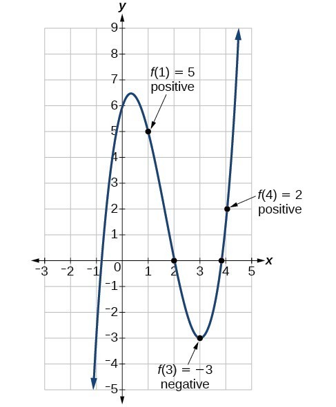
• Convergence in numerical analysis approaches a specific value or solution as the number of iterations increases
• Bisection method converges to a root of a continuous function f(x) on an interval [a,b] where f(a) and f(b) have opposite signs
• Intermediate Value Theorem guarantees convergence by stating a continuous function must cross the x-axis between two points with opposite signs
• Sequence of intervals generated by the bisection method forms a nested sequence converging to the root
• Linear convergence characterizes the bisection method, approximately halving the error in each iteration
• Rate of convergence expressed as $|x_{n+1} - r| \leq (1/2)|x_n - r|$, where $x_n$ is the nth approximation and r is the true root

Mathematical Properties and Implications

• Bisection method always converges for continuous functions on a given interval
• Convergence rate remains constant regardless of the function's behavior (unlike Newton's method)
• Guaranteed convergence makes bisection method valuable for initializing faster methods
• Slow convergence can be a drawback for high-precision requirements or computationally expensive functions
• Linear convergence implies doubling iterations to gain one additional digit of accuracy
• Reliability of bisection method compensates for its slower convergence in certain scenarios (highly nonlinear functions)

Iterations for Desired Accuracy

Deriving the Iteration Formula

• Formula for number of iterations (n) derived from relationship between initial interval length and desired accuracy
• Initial interval length (b - a) where a and b are endpoints of starting interval
• After n iterations, interval length reduced to $(b - a) / 2^n$
• To achieve desired accuracy ε, we need $(b - a) / 2^n \leq \varepsilon$
• Taking logarithm of both sides and solving for n yields formula: $n \geq \log_2((b - a) / \varepsilon)$
• Ceiling function applied to ensure integer number of iterations: $n = \lceil\log_2((b - a) / \varepsilon)\rceil$
• This formula provides minimum number of iterations required to guarantee an error less than or equal to ε

Practical Applications and Considerations

• Formula allows pre-determination of computational cost for desired accuracy
• Useful for resource allocation in time-sensitive applications (real-time systems)
• Helps in comparing efficiency with other root-finding methods for specific problems
• Can be used to set appropriate maximum iteration limits in implementation
• Demonstrates logarithmic relationship between accuracy and number of iterations
• Illustrates trade-off between precision and computational time in numerical methods

Rate of Convergence Analysis

Characteristics of Linear Convergence

• Bisection method exhibits linear convergence with order of convergence equal to 1
• Error reduction factor is 1/2, approximately halving error in each iteration
• Convergence rate expressed as $|e_{n+1}| \leq C|e_n|$, where $e_n$ is error at nth iteration and C is constant (1/2 for bisection)
• Linear convergence requires doubling iterations to gain one additional digit of accuracy
• Slow convergence rate can be disadvantageous for high-precision requirements
• Computationally expensive functions may make bisection method less efficient compared to faster-converging methods

Comparative Analysis and Implications

• Despite slow convergence, bisection method's reliability makes it valuable for certain applications
• Useful for initializing faster methods (Newton's method) that require good initial guesses
• Effective for problems where other methods may fail due to function behavior (highly nonlinear functions)
• Constant convergence rate regardless of function complexity provides predictable performance
• Trade-off between reliability and speed often favors bisection method in robust algorithm design
• Understanding convergence rate crucial for selecting appropriate method for specific problem requirements

Error Bounds and Stopping Criteria

Error Estimation Techniques

• Maximum error after n iterations given by $(b - a) / 2^{(n+1)}$, where (b - a) is initial interval length
• A priori error estimation uses formula $|x_n - r| \leq (b - a) / 2^n$, where $x_n$ is nth approximation and r is true root
• Relative error estimated as $|(x_{n+1} - x_n) / x_{n+1}|$, providing practical stopping criterion
• Error bounds help in assessing accuracy of approximation at any iteration
• Estimation techniques allow for adaptive iteration control in implementation
• Understanding error behavior crucial for balancing accuracy and computational efficiency

Implementing Effective Stopping Criteria

• Common stopping criteria include reaching maximum number of iterations (prevents infinite loops)
• Achieving desired tolerance ε (based on absolute or relative error)
• Condition $|f(x_n)| < \delta$ for small δ (indicates proximity to root)
• Choice of stopping criteria affects balance between accuracy and computational efficiency
• Roundoff errors in floating-point arithmetic can limit achievable accuracy
• Consideration of machine epsilon necessary in setting realistic error bounds
• Multiple criteria often combined for robust implementation (maximum iterations as failsafe)

Bisection Method vs Other Algorithms

Convergence Rate Comparison

• Bisection method has linear convergence (order 1)
• Newton's method exhibits quadratic convergence (order 2) when it converges
• Secant method demonstrates superlinear convergence (order ≈ 1.618)
• Fixed-point iteration methods have varying convergence rates depending on chosen function
• Newton's method typically requires fewer iterations than bisection for same accuracy
• Secant method converges faster than bisection but slower than Newton's method

Reliability and Applicability Analysis

• Bisection method guarantees convergence for continuous functions, more reliable than Newton's method
• Newton's method can fail to converge for certain initial guesses or function behaviors (flat regions)
• Secant method doesn't require derivative calculation, advantageous for complex functions
• Fixed-point methods can be faster than bisection when they converge, but may diverge in some cases
• Hybrid methods (Brent's method) combine reliability of bisection with speed of higher-order methods
• Choice of method depends on function characteristics, desired accuracy, and computational constraints