Gradient descent is a key optimization technique in neural networks, helping find the best parameters to minimize errors. It works by adjusting weights and biases based on calculated gradients, moving towards lower error rates with each iteration.
Various gradient descent methods exist, from batch to stochastic approaches. These techniques, along with momentum-based and adaptive learning rate methods, aim to improve convergence speed and stability in the complex landscape of neural network optimization.
Gradient Descent for Optimization
Understanding Gradient Descent
- Gradient descent is an optimization algorithm used to minimize the cost function of a neural network by iteratively adjusting the model's parameters (weights and biases) in the direction of steepest descent of the cost function
- The goal of gradient descent is to find the optimal set of parameters that minimize the difference between the predicted outputs and the actual outputs, thereby improving the neural network's performance
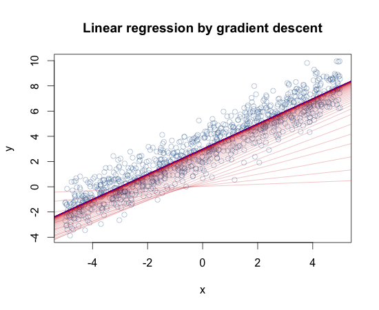
- Gradient descent calculates the gradient of the cost function with respect to each parameter and updates the parameters in the opposite direction of the gradient, gradually moving towards the minimum of the cost function
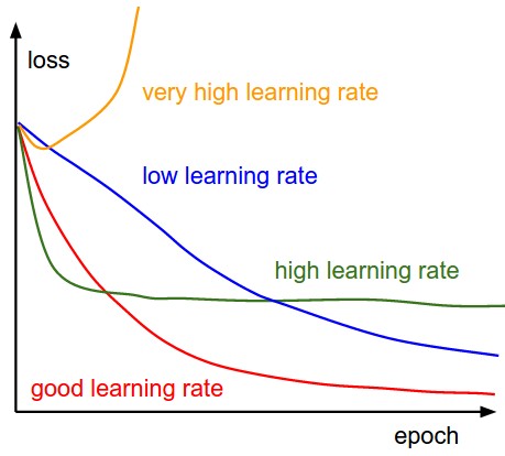
- The learning rate is a hyperparameter that determines the step size at which the parameters are updated in each iteration of gradient descent, controlling the speed of convergence
Challenges in Gradient Descent
- Gradient descent can be prone to getting stuck in local minima, saddle points, or plateaus, which are suboptimal solutions where the cost function is not the global minimum
- Local minima are points where the cost function is lower than the surrounding points but higher than the global minimum, causing gradient descent to converge to a suboptimal solution
- Saddle points are points where the cost function has zero gradient but is not a minimum, causing gradient descent to slow down or stop prematurely
- Plateaus are flat regions in the cost function landscape where the gradient is close to zero, making it difficult for gradient descent to make progress and leading to slow convergence
Gradient Descent Techniques
Batch, Stochastic, and Mini-Batch Gradient Descent
- Batch gradient descent, also known as vanilla gradient descent, computes the gradient of the cost function using the entire training dataset in each iteration, making it computationally expensive for large datasets and slower to converge
- Stochastic gradient descent (SGD) updates the model's parameters based on the gradient calculated from a single, randomly selected training example in each iteration, making it faster and more suitable for large datasets but with higher variance in the updates
- Mini-batch gradient descent strikes a balance between batch and stochastic gradient descent by dividing the training dataset into smaller batches and computing the gradient based on each mini-batch, providing a trade-off between convergence speed and computational efficiency
Momentum-Based and Adaptive Learning Rate Methods
- Momentum-based optimization techniques, such as classical momentum and Nesterov accelerated gradient (NAG), introduce a momentum term that accumulates past gradients to smooth out oscillations and accelerate convergence in relevant directions
- Classical momentum adds a fraction of the previous update vector to the current update, helping to maintain a consistent direction and overcome small local minima or plateaus
- Nesterov accelerated gradient (NAG) calculates the gradient at a point ahead of the current position in the direction of the momentum, allowing for more accurate updates and faster convergence
- Adaptive learning rate methods, like AdaGrad, RMSprop, and Adam, adjust the learning rate for each parameter based on its historical gradients, allowing for faster convergence and better handling of sparse gradients
- AdaGrad adapts the learning rate for each parameter inversely proportional to the square root of the sum of its historical squared gradients, giving larger updates to infrequent parameters and smaller updates to frequent parameters
- RMSprop is an extension of AdaGrad that uses an exponentially decaying average of squared gradients to reduce the aggressive learning rate decay
- Adam (Adaptive Moment Estimation) combines the benefits of momentum and adaptive learning rates by maintaining both the first and second moments of the gradients, providing a robust and efficient optimization algorithm
Error Minimization with Gradient Descent
Error Functions and Backpropagation
- The error function, also known as the cost function or loss function, quantifies the difference between the predicted outputs and the actual outputs of a neural network, serving as a measure of the model's performance
- Common error functions for regression problems include mean squared error (MSE) and mean absolute error (MAE), while cross-entropy loss is often used for classification tasks
- Mean squared error (MSE) calculates the average squared difference between the predicted and actual values:
- Mean absolute error (MAE) calculates the average absolute difference between the predicted and actual values:
- Cross-entropy loss measures the dissimilarity between the predicted probability distribution and the true probability distribution, commonly used in binary and multi-class classification problems
- Gradient descent minimizes the error function by iteratively updating the model's parameters in the direction of the negative gradient of the error function with respect to each parameter
- The update rule for gradient descent is given by:
θ_new = θ_old - α * ∇J(θ), whereθrepresents the parameters,αis the learning rate, and∇J(θ)is the gradient of the error function with respect to the parameters - Backpropagation is an algorithm used to efficiently compute the gradients of the error function with respect to the weights and biases in a neural network by applying the chain rule of calculus
Convergence and Stability of Gradient Descent
Factors Affecting Convergence
- Convergence of gradient descent refers to the property of the algorithm to reach a minimum of the cost function, ideally the global minimum, within a reasonable number of iterations
- The learning rate plays a crucial role in the convergence of gradient descent: too small a learning rate leads to slow convergence, while too large a learning rate can cause the algorithm to overshoot the minimum and diverge
- The choice of initialization for the model's parameters can affect the convergence of gradient descent, with techniques like Xavier initialization and He initialization helping to mitigate the vanishing and exploding gradient problems
- Xavier initialization sets the initial weights to random values drawn from a uniform distribution with a variance that depends on the number of input and output units in each layer, promoting stable gradients and faster convergence
- He initialization is similar to Xavier initialization but is designed for rectified linear unit (ReLU) activation functions, setting the initial weights to random values drawn from a normal distribution with a variance that depends on the number of input units
Techniques for Improving Stability
- Batch normalization is a technique that normalizes the activations of each layer in a neural network, helping to stabilize the training process and improve the convergence of gradient descent
- Batch normalization reduces the internal covariate shift by normalizing the inputs to each layer, allowing for higher learning rates and faster convergence while also acting as a regularizer
- Early stopping is a regularization technique that monitors the model's performance on a validation set during training and stops the gradient descent process when the performance starts to degrade, preventing overfitting and promoting better generalization
- Early stopping helps to find the optimal point at which the model has learned the underlying patterns in the data without memorizing noise or irrelevant features
- Gradient clipping is a technique used to limit the magnitude of gradients to a specific range, helping to stabilize the training process and prevent the gradients from becoming too large, which can lead to unstable updates
- Gradient clipping can be applied by scaling the gradients to a maximum threshold (L∞ norm clipping) or by scaling the gradients such that their L2 norm is within a specified limit (L2 norm clipping)