Steepest descent is a fundamental optimization method that moves towards the minimum of a function by following the . It's simple yet powerful, making it a cornerstone of many optimization algorithms used in machine learning and other fields.

While steepest descent can be effective, it has limitations. It may converge slowly for and struggle with saddle points. Understanding its strengths and weaknesses is crucial for applying it effectively and knowing when to use more advanced gradient-based methods.

Steepest Descent Optimization

Concept and Motivation

Top images from around the web for Concept and Motivation
  • iteratively finds of differentiable functions
  • Moves in direction of negative gradient representing steepest descent at each point
  • Updates current solution by taking steps proportional to negative gradient
  • Useful for unconstrained optimization problems with continuous, differentiable objective functions
  • Simplicity and low computational cost per iteration make it attractive for large-scale problems
  • Applies to both convex and non-convex optimization problems (may converge to local minima in non-convex cases)
  • Assumes moving in direction of steepest descent leads to function minimum

Applications and Considerations

  • Particularly effective for quadratic or nearly quadratic objective functions
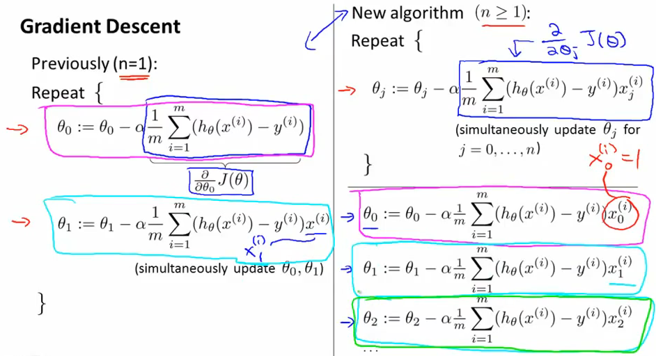
  • Widely used in machine learning for training neural networks ()
  • Applied in image processing for denoising and image reconstruction
  • Utilized in control systems for parameter optimization
  • Employed in financial modeling for portfolio optimization
  • Considerations when using steepest descent
    • Function landscape (, smoothness)
    • Problem dimensionality
    • Computational resources available
    • Required accuracy of solution

Implementing Steepest Descent

Algorithm Components

  • Compute gradient of at each iteration
  • Select initial starting point (random initialization or domain-specific heuristics)
  • Specify stopping criterion (maximum iterations or change in function value tolerance)
  • Determine step size () affecting convergence
    • Fixed step sizes (simple but may lead to slow convergence)
    • methods (, trust region strategies)
  • Basic update rule xk+1=xkαkf(xk)x_{k+1} = x_k - \alpha_k \nabla f(x_k)
    • xkx_k current point
    • αk\alpha_k step size
    • f(xk)\nabla f(x_k) gradient at xkx_k

Implementation Techniques

  • Approximate gradients using (finite difference methods)
  • Include safeguards against numerical instabilities
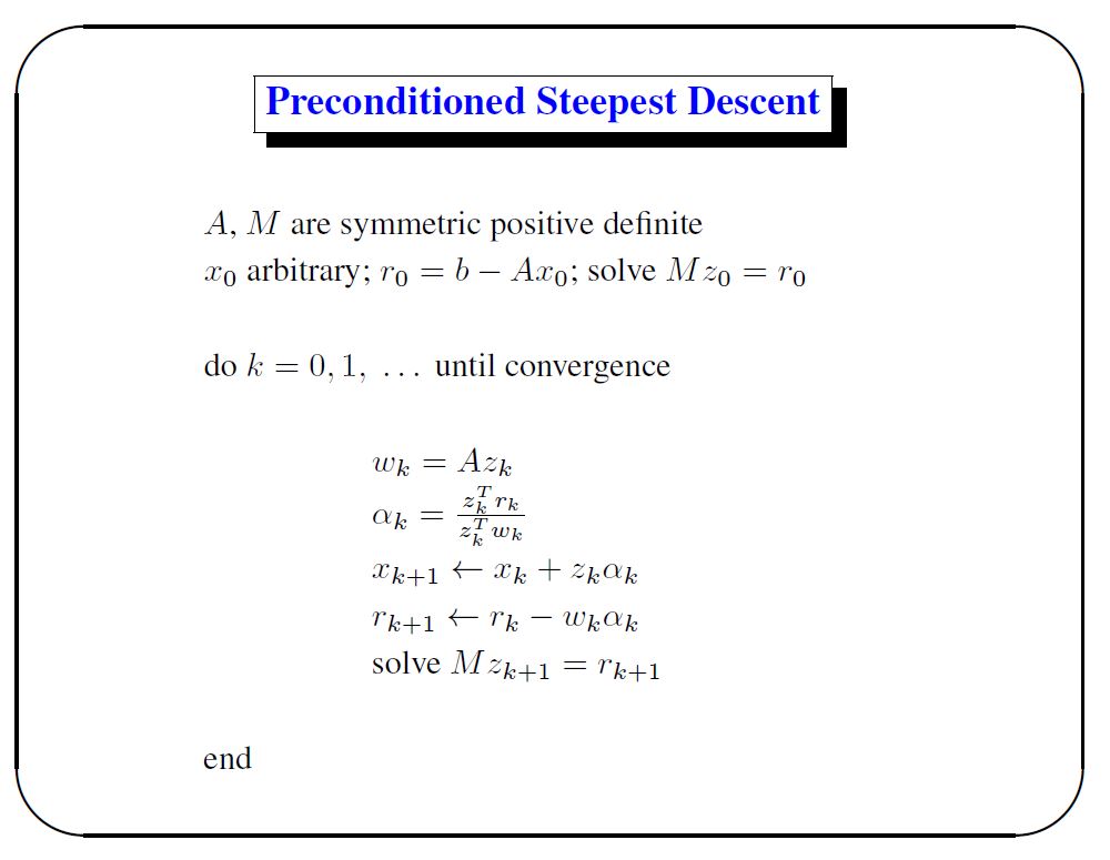
  • Handle ill-conditioned problems (preconditioning, regularization)
  • Use vectorized implementations for high-dimensional problems
  • Implement backtracking line search for adaptive step size
    • Start with large step size
    • Reduce until sufficient decrease condition met
  • Incorporate to accelerate convergence
  • Implement to prevent overfitting in machine learning applications

Convergence Properties of Steepest Descent

Convergence Characteristics

  • Linear (slower than higher-order methods)
  • Guaranteed convergence for strictly convex functions with Lipschitz continuous gradients
  • Zigzag phenomenon slows convergence in ill-conditioned problems
    • Takes steps nearly orthogonal to optimal direction
    • Results in inefficient path to optimum
  • Performance sensitive to objective function scaling
  • Convergence rate depends on condition number at optimum
  • Quadratic functions worst-case convergence rate related to Hessian eigenvalue ratio
  • Struggles with saddle points and plateau regions

Factors Affecting Convergence

  • Initial starting point selection impacts convergence speed
  • Step size choice critical for balancing convergence speed and stability
    • Too large may cause overshooting and divergence
    • Too small leads to slow convergence
  • Problem dimensionality affects convergence rate
    • Higher dimensions generally require more iterations
  • Function curvature influences convergence behavior
    • Highly curved regions may cause slow progress
  • Noise in gradient estimates can impact convergence ()

Steepest Descent vs Other Techniques

Comparison with Newton's Method

  • Steepest descent less efficient than for smooth, well-conditioned problems
  • Newton's method requires second-order derivative information (Hessian matrix)
  • Steepest descent more suitable for large-scale problems where Hessian computation prohibitive
  • Newton's method converges quadratically near optimum, steepest descent linearly
  • Steepest descent more robust to initial point selection

Comparison with Other Gradient-Based Methods

  • Conjugate gradient methods often outperform steepest descent
    • Use information from previous iterations to improve search direction
    • Particularly effective for quadratic functions
  • Momentum-based variants improve convergence rates
    • Heavy ball method adds momentum term to update rule
    • Nesterov's accelerated gradient uses "look-ahead" step
  • Stochastic preferred for large-scale machine learning
    • Handles noisy gradients and large datasets efficiently
    • Mini-batch processing allows for frequent updates

Applicability to Different Problem Types

  • Steepest descent effective for smooth, unconstrained optimization
  • Subgradient methods more appropriate for non-smooth optimization
  • Proximal gradient methods handle composite optimization problems
  • Trust region methods provide better global convergence properties
  • Quasi-Newton methods (BFGS, L-BFGS) offer superlinear convergence without explicit Hessian computation

Key Terms to Review (25)

Adaptive step size: Adaptive step size refers to a technique used in optimization algorithms where the step length is adjusted dynamically based on the current state of the algorithm. This approach helps to improve convergence rates by allowing larger steps when close to a solution and smaller steps when farther away, ensuring a more efficient search process. The method is particularly relevant in iterative techniques where the behavior of the objective function is uncertain or highly variable.
Backpropagation: Backpropagation is an algorithm used for training artificial neural networks by calculating the gradient of the loss function with respect to each weight by the chain rule, enabling efficient weight updates. This method is crucial in optimizing the network's performance by minimizing the error between predicted and actual outcomes, leading to improved learning over multiple iterations.
Convergence criteria: Convergence criteria are specific conditions or thresholds used to determine when an iterative optimization algorithm has successfully reached a solution that is sufficiently close to the optimal result. These criteria help in evaluating the progress of the algorithm and ensure that further iterations are either unnecessary or unlikely to yield significant improvement.
Convergence Rate: The convergence rate refers to the speed at which an iterative optimization algorithm approaches its solution. It is crucial in understanding how quickly a method can find an optimal solution and can vary significantly between different algorithms, influencing their efficiency and practicality in solving optimization problems.
Convexity: Convexity refers to a property of a set or a function where, for any two points within the set or on the function, the line segment connecting these points lies entirely within the set or above the function. This characteristic is crucial in optimization as it simplifies the analysis of feasible regions, objective functions, and constraints, leading to more efficient solution methods.
Early stopping: Early stopping is a technique used in optimization to prevent overfitting by halting the training process of an algorithm before it reaches its maximum potential. This method relies on monitoring the performance of the algorithm on a validation dataset, allowing it to stop when performance begins to degrade, rather than improving. By implementing early stopping, one can maintain a balance between underfitting and overfitting, ensuring the model generalizes well to unseen data.
Fixed step size: A fixed step size refers to a predetermined, constant amount used in optimization algorithms to determine the step length taken in each iteration. This method simplifies the process of finding a minimum by consistently applying the same distance in the direction of the steepest descent, which can streamline calculations and implementation in iterative methods.
Gradient Descent: Gradient descent is an optimization algorithm used to minimize a function by iteratively moving towards the steepest descent, which is determined by the negative gradient of the function at a given point. This method is essential in identifying the best parameters in various fields, including mathematical modeling, machine learning, and engineering design optimization.
Gradient vector: A gradient vector is a multi-variable generalization of a derivative, representing the direction and rate of fastest increase of a scalar function. It is a crucial tool in optimization problems, as it helps determine the steepest ascent or descent direction in the context of functions with multiple variables.
Hessian Matrix: The Hessian matrix is a square matrix of second-order partial derivatives of a scalar-valued function, providing important information about the curvature of the function's graph. It is critical in optimization as it helps determine the nature of critical points, indicating whether they are local minima, local maxima, or saddle points based on its eigenvalues.
Ill-conditioned problems: Ill-conditioned problems are mathematical optimization scenarios where small changes in the input can lead to large changes in the output, making them unstable and difficult to solve accurately. These problems typically arise in numerical analysis, especially when dealing with steepest descent methods, where the direction of descent can be significantly affected by slight perturbations in the data or initial conditions.
Iteration step: An iteration step is a single update or move in the process of finding a solution to an optimization problem, typically involving adjustments based on the current estimate of the solution. Each iteration step aims to improve the current estimate by moving towards a more optimal solution, utilizing information like gradients or directions derived from the objective function. This concept is central to optimization methods, particularly those that rely on iterative processes to converge on a solution.
Learning Rate: The learning rate is a hyperparameter that determines the step size at each iteration while moving toward a minimum of a loss function. It plays a crucial role in optimization algorithms, influencing how quickly or slowly a model learns from the data. A properly set learning rate can greatly enhance convergence speed and model performance, while an incorrect setting can lead to overshooting the optimal solution or slow convergence.
Line search: Line search is a numerical optimization technique used to find a suitable step size along a given search direction that minimizes an objective function. It serves as a crucial component in various optimization algorithms, helping to ensure efficient convergence to a local minimum by determining how far to move in the direction of the negative gradient or other search directions. The effectiveness of line search can significantly influence the performance of optimization methods.
Lipschitz Continuity: Lipschitz continuity is a property of a function that ensures the difference in function values is bounded by a constant multiple of the difference in input values. This means that if you change your input a little, the output won’t change too much, making it an important concept for analyzing the behavior of functions. Lipschitz continuity helps establish stability in optimization problems, convergence rates in algorithms, and guarantees on the solutions, particularly when dealing with convex functions and gradient-based methods.
Local minima: Local minima refer to points in a function where the value is lower than that of its neighboring points, indicating a potential minimum in the vicinity. These points are important in optimization as they represent values that can be used to evaluate the performance of an algorithm. Understanding local minima is crucial for techniques that aim to find optimal solutions, especially when the landscape of the function is complex.
Momentum terms: Momentum terms refer to components in optimization algorithms that help accelerate convergence by incorporating previous gradient information. These terms essentially provide a memory effect that can improve the efficiency and speed of the optimization process, particularly in methods like steepest descent where gradient information is utilized iteratively. By combining current gradient data with past updates, momentum terms can help navigate the optimization landscape more effectively.
Negative gradient: The negative gradient is a vector that points in the direction of the steepest descent of a function, representing the greatest rate of decrease of that function. This concept is crucial in optimization methods, particularly when searching for local minima, as it indicates how to adjust variables to minimize a function effectively.
Newton's Method: Newton's Method is an iterative numerical technique used to find approximate solutions to optimization problems, particularly for identifying critical points of differentiable functions. This method employs the first and second derivatives of a function to refine guesses about the location of these points, making it highly efficient for unconstrained optimization tasks.
Numerical techniques: Numerical techniques refer to a set of mathematical methods and algorithms used to approximate solutions for complex mathematical problems that may not have exact solutions. These methods are particularly useful in optimization, where finding the best solution often requires iterative approaches to navigate through large solution spaces. Numerical techniques allow for the practical application of mathematics in various fields, including engineering, economics, and data science, making them essential tools for solving real-world problems.
Objective Function: An objective function is a mathematical expression that defines the goal of an optimization problem, representing either a maximization or minimization task. It is typically formulated as a function of decision variables, which are the unknowns that need to be determined in order to achieve the best outcome based on given constraints.
Partial Derivative: A partial derivative is a derivative where only one variable is differentiated while keeping the other variables constant. This concept is crucial when dealing with functions of multiple variables, allowing us to understand how the function changes with respect to one variable at a time. In optimization, partial derivatives are used to find the direction in which a function increases or decreases, which is essential for methods like steepest descent.
Smoothness Condition: The smoothness condition refers to a property of functions that ensures they are continuously differentiable, which is crucial for the convergence of optimization algorithms. This property guarantees that the gradient of the function does not change too abruptly, enabling methods such as steepest descent to effectively navigate towards local minima. Smoothness conditions often relate to concepts such as Lipschitz continuity, which further characterizes how functions behave in the vicinity of their input values.
Steepest descent method: The steepest descent method is an iterative optimization algorithm used to find the minimum of a differentiable function by moving in the direction of the steepest decrease of the function. This method utilizes the gradient of the function, which points in the direction of the greatest rate of increase, and hence, the negative gradient indicates the direction of steepest descent. By taking steps proportional to this negative gradient, the algorithm converges towards a local minimum, making it an essential technique in optimization problems.
Stochastic settings: Stochastic settings refer to situations or models that incorporate randomness and uncertainty, where outcomes are influenced by probabilistic factors. In optimization, understanding stochastic settings is crucial as it allows for the formulation of models that can address real-world problems with inherent variability, enabling decision-making under uncertainty.
© 2024 Fiveable Inc. All rights reserved.
AP® and SAT® are trademarks registered by the College Board, which is not affiliated with, and does not endorse this website.