2.3 Estimate a Variable and Fixed Cost Equation and Predict Future Costs

3 min readjune 18, 2024

Estimating variable and fixed costs is crucial for understanding how expenses change with activity levels. The and scatter graphs help managers analyze and create cost equations for predicting future expenses.

These tools enable businesses to make informed decisions about pricing, resource allocation, and capacity planning. By accurately estimating costs, companies can better forecast budgets, perform , and evaluate the impact of changing activity levels on total costs.

Estimating Variable and Fixed Costs

High-low method for cost estimation

Top images from around the web for High-low method for cost estimation
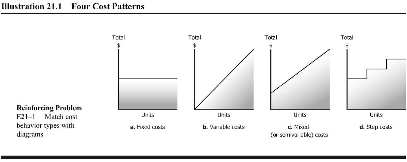
  • contain both variable and fixed cost elements (labor costs with overtime pay)
  • estimates variable and fixed components of
  • Identify periods with highest and lowest activity levels (, units produced)
  • Determine total costs for highest and lowest activity periods
  • Calculate using formula: Variable cost per unit=Highest total costLowest total costHighest activity levelLowest activity level\text{Variable cost per unit} = \frac{\text{Highest total cost} - \text{Lowest total cost}}{\text{Highest activity level} - \text{Lowest activity level}}
  • Calculate total fixed cost using highest or lowest activity level and corresponding total cost: Total fixed cost=Total cost at highest or lowest activity level(Variable cost per unit×Corresponding activity level)\text{Total fixed cost} = \text{Total cost at highest or lowest activity level} - (\text{Variable cost per unit} \times \text{Corresponding activity level})
  • Resulting : Total cost=Fixed cost+(Variable cost per unit×Activity level)\text{Total cost} = \text{Fixed cost} + (\text{Variable cost per unit} \times \text{Activity level})
  • Predict future costs by inputting different activity levels into (production volumes, service hours)
  • Consider the when applying the cost equation to ensure accuracy

Scatter graphs and cost relationships

  • visually represents relationship between costs and activity levels
  • Activity levels plotted on x-axis (labor hours, units produced)
  • Total costs plotted on y-axis
  • Each data point represents total cost at specific activity level
  • suggests linear relationship between costs and activity
    • Straight line approximates cost behavior (upward sloping for increasing costs)
  • indicates cost behavior is not linear
    • High-low method may not be appropriate (curvilinear, exponential relationships)
  • Scatter graphs help identify that influence total costs

Cost equations in business applications

  • Cost equation from high-low method calculates total costs at different activity levels Total cost=Fixed cost+(Variable cost per unit×Activity level)\text{Total cost} = \text{Fixed cost} + (\text{Variable cost per unit} \times \text{Activity level})
  • Manufacturing businesses:
    • Activity levels include machine hours, labor hours, units produced
    • Estimate total production costs at different output levels (batch sizes, production runs)
  • Service businesses:
    • Activity levels include service hours, customers served, transactions processed
    • Estimate total service costs at different activity levels (consulting projects, customer support)
  • Managers use cost equations to:
    1. Predict future costs based on expected activity (budgeting, forecasting)
    2. Make decisions on pricing, resource allocation, capacity planning (break-even analysis)
    3. Evaluate impact of activity level changes on total costs ()

Advanced Cost Estimation Techniques

  • provides a more sophisticated method for estimating cost equations
  • minimizes the sum of squared differences between actual and predicted costs
  • Cost behavior patterns can be analyzed to understand how costs change with activity levels
  • Identifying appropriate cost drivers is crucial for accurate cost estimation and decision-making

Key Terms to Review (22)

Break-Even Analysis: Break-even analysis is a fundamental concept in managerial accounting that determines the point at which a company's total revenue equals its total costs, meaning the company has neither a profit nor a loss. It is a valuable tool for understanding the relationship between a company's fixed costs, variable costs, and sales volume, and for making informed decisions about pricing, production, and profitability.
Cost Behavior: Cost behavior refers to the relationship between a company's costs and its level of business activity or output. It describes how different types of costs, such as variable costs and fixed costs, respond to changes in the volume of production or sales.
Cost behaviors: Cost behaviors describe how costs change in relation to changes in a company's level of activity. These behaviors are essential for budgeting, forecasting, and decision-making processes.
Cost Drivers: Cost drivers are the factors that directly influence the incurrence of costs within an organization. They are the underlying causes that determine the level of resources consumed and the resulting costs associated with business activities or operations. Cost drivers play a crucial role in various managerial accounting concepts, including the estimation of variable and fixed costs, the application of job order and process costing methods, the calculation of activity-based product costs, and the analysis of overhead variances.
Cost equation: A cost equation is a mathematical formula used to predict total costs by summing variable and fixed costs. It typically takes the form: Total Cost = Fixed Costs + (Variable Cost per Unit × Number of Units).
Cost Equation: The cost equation is a mathematical model that represents the relationship between a company's total costs, fixed costs, and variable costs. It is a fundamental tool used in managerial accounting to estimate and predict future costs based on changes in activity levels.
High-low method: The high-low method is a technique used to estimate the fixed and variable components of a cost by analyzing the highest and lowest activity levels. It helps in creating a cost equation that can predict future costs based on expected activity levels.
High-Low Method: The high-low method is a technique used to estimate the variable and fixed components of a mixed cost by analyzing the relationship between the total cost and the activity level. It helps determine the fixed and variable portions of a cost based on the highest and lowest levels of activity observed.
Least Squares Method: The least squares method is a statistical technique used to estimate the parameters of a linear equation that best fits a set of data points. It aims to minimize the sum of the squared differences between the observed values and the predicted values from the linear equation.
Linear Pattern: A linear pattern refers to a relationship between two variables where the change in one variable is directly proportional to the change in the other variable. This type of pattern is commonly observed in cost behavior analysis and is crucial for estimating variable and fixed cost equations as well as predicting future costs.
Machine Hours: Machine hours refer to the total number of hours that a production machine is in operation during a specific period. This metric is crucial in various managerial accounting contexts, as it helps understand and analyze the relationship between machine usage, costs, and production efficiency.
Mixed costs: Mixed costs are expenses that have both fixed and variable components. These costs change with production levels but not proportionally.
Mixed Costs: Mixed costs are a type of cost that contain both a fixed and a variable component. They are expenses that change in total as the level of activity changes, but not proportionally. Mixed costs have a fixed portion that remains constant regardless of activity, and a variable portion that fluctuates with changes in activity.
Non-Linear Pattern: A non-linear pattern refers to a relationship between variables that does not follow a straight line or linear trend. In the context of cost estimation and prediction, a non-linear pattern indicates that the relationship between the independent variable (such as volume or activity) and the dependent variable (such as cost) is not constant or proportional.
Regression Analysis: Regression analysis is a statistical technique used to model and analyze the relationship between a dependent variable and one or more independent variables. It is a powerful tool for estimating and predicting future values based on observed data.
Relevant range: The relevant range is the span of activity levels within which specific cost behaviors are valid. Outside this range, fixed and variable cost estimates may not hold true.
Relevant Range: The relevant range is a concept in managerial accounting that refers to the range of activity levels over which certain assumptions about cost behavior can be considered valid. It is a critical factor in understanding and predicting cost behavior patterns, estimating variable and fixed cost equations, comparing costing methods, and preparing flexible budgets.
Scatter graph: A scatter graph is a visual representation of the relationship between two variables using Cartesian coordinates. It plots individual data points to help identify trends or patterns, such as linear relationships in cost behavior analysis.
Scatter Graph: A scatter graph, also known as a scatter plot, is a type of visual representation that displays the relationship between two variables by plotting individual data points on a coordinate plane. It is commonly used in the context of estimating variable and fixed cost equations, as well as predicting future costs.
Sensitivity analysis: Sensitivity analysis evaluates how different values of an independent variable affect a particular dependent variable under a given set of assumptions. It's used to predict the outcome of a decision given a certain range of variables in managerial accounting.
Sensitivity Analysis: Sensitivity analysis is a technique used to assess the impact of changes in one or more input variables on the output or outcome of a model or decision. It helps understand how sensitive the results are to variations in the assumptions or inputs, allowing decision-makers to identify the most critical factors and make informed choices.
Variable Cost per Unit: The variable cost per unit refers to the cost that varies directly with the level of production or service output. It represents the additional cost incurred for producing or providing one more unit of a product or service.
© 2024 Fiveable Inc. All rights reserved.
AP® and SAT® are trademarks registered by the College Board, which is not affiliated with, and does not endorse this website.