Finite difference and finite volume methods are crucial numerical techniques for solving MHD equations. They discretize continuous equations into algebraic forms, allowing us to simulate complex plasma behaviors on computers.

These methods differ in their approach to discretization and conservation properties. Finite difference approximates derivatives directly, while finite volume ensures conservation of physical quantities, making it better suited for problems with shocks and discontinuities.

Finite Difference Methods in MHD

Principles and Approximations

Top images from around the web for Principles and Approximations
  • Finite difference methods approximate derivatives in MHD equations using discrete grid points replacing continuous differential equations with algebraic equations
  • discretizes spatial derivatives while keeping time continuous reducing PDEs to systems of ODEs
  • Common approximation schemes include
  • Each scheme offers specific advantages and limitations in MHD simulations
  • Particularly useful for solving and in MHD allowing evolution of magnetic fields and fluid velocities
  • Grid spacing and time step choice significantly impacts accuracy and stability often governed by

Advanced Techniques and Considerations

  • (fourth-order, sixth-order) provide improved accuracy at cost of increased computational complexity
  • Spatial derivatives approximated using Taylor series expansions of neighboring points
  • (Runge-Kutta, Adams-Bashforth) used to advance solution in time
  • often employed to avoid checkerboard instabilities in MHD simulations
  • or may be added to stabilize simulations of highly nonlinear MHD phenomena
  • Boundary conditions require special treatment often using or

Finite Volume Methods for MHD

Conservation Laws and Discretization

  • Finite volume methods discretize integral form of conservation laws ensuring global conservation of mass, momentum, and energy in MHD simulations
  • Domain divided into with calculated at interfaces between volumes to update conserved quantities
  • (, ) handle discontinuities and shocks in MHD flows
  • and maintain positivity and prevent spurious oscillations
  • maintain of magnetic field (B=0\nabla \cdot \mathbf{B} = 0) to machine precision
  • increases resolution in regions of interest while maintaining computational efficiency

Advanced Techniques and Applications

  • widely used for solving MHD equations in conservative form
  • MUSCL (Monotonic Upstream-centered Scheme for Conservation Laws) reconstruction improves spatial accuracy
  • (HLL, HLLD) balance accuracy and computational efficiency
  • (minmod, van Leer) prevent oscillations near discontinuities
  • handle multidimensional MHD problems more accurately than dimensional splitting
  • can improve efficiency for problems with varying characteristic speeds

Finite Difference vs Finite Volume

Fundamental Differences

  • Finite difference methods operate on differential form of MHD equations while finite volume methods work with integral form
  • Finite volume methods naturally ensure conservation of physical quantities suitable for problems with shocks and discontinuities
  • Finite difference methods offer simpler implementation and lower computational cost but may struggle with conservation in complex MHD flows
  • Boundary condition implementation more straightforward in finite difference methods
  • Finite volume methods better suited for irregular geometries and unstructured grids

Method Selection and Applications

  • Choice between methods depends on specific MHD problem
  • Finite volume methods preferred for compressible MHD (stellar atmospheres, accretion disks)
  • Finite difference methods suited for incompressible or simplified MHD models (planetary magnetospheres, solar corona)
  • Hybrid approaches combining finite difference and finite volume techniques exist for specialized MHD applications
  • Spectral methods offer alternative approach with high accuracy for smooth solutions but struggle with discontinuities

Stability, Accuracy, and Convergence of MHD Methods

Stability Analysis and Theorems

  • assesses stability of finite difference and finite volume schemes particularly for linear problems
  • states for consistent finite difference schemes stability necessary and sufficient for convergence as grid refined
  • CFL condition provides necessary (not always sufficient) condition for stability of explicit time-stepping schemes
  • Total Variation Diminishing (TVD) schemes ensure total variation of numerical solution does not increase over time providing measure of stability for nonlinear MHD problems

Accuracy and Convergence Properties

  • Order of accuracy determined by in Taylor series expansion of discretized equations
  • Convergence rates for smooth solutions typically follow O(Δxp+Δtq)O(\Delta x^p + \Delta t^q) where p and q are spatial and temporal orders of accuracy
  • Discontinuities or shocks in MHD flows can reduce convergence rate necessitating special treatment (shock-capturing schemes)
  • Richardson extrapolation used to estimate discretization errors and improve solution accuracy
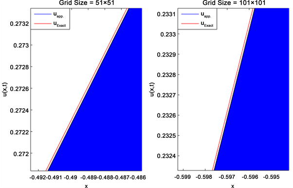
  • Grid convergence studies essential for verifying numerical results in MHD simulations
  • Implicit methods often provide better stability properties allowing larger time steps at cost of increased computational complexity per step

Key Terms to Review (56)

Adams-Bashforth Method: The Adams-Bashforth method is a family of explicit multistep methods used for numerically solving ordinary differential equations. It leverages previously computed values of the solution to estimate future values, making it efficient for time-stepping problems. This method is particularly useful in contexts like finite difference and finite volume methods, where the solution evolves over time and must be approximated accurately at discrete intervals.
Adaptive mesh refinement (AMR): Adaptive mesh refinement (AMR) is a computational technique used to dynamically adjust the resolution of a grid or mesh in numerical simulations based on the solution's features and requirements. This method allows for finer resolution in areas with complex phenomena while maintaining coarser grids in regions with less activity, optimizing computational resources and enhancing accuracy.
Approximate Riemann Solvers: Approximate Riemann solvers are numerical methods used to solve hyperbolic partial differential equations by approximating the solution to the Riemann problem at cell interfaces. These solvers are crucial for computational fluid dynamics and magnetohydrodynamics, as they provide a way to handle discontinuities in the flow, such as shock waves, by estimating the flux across interfaces using simplified models. The balance between accuracy and computational efficiency is a key feature of these solvers, making them widely applicable in finite difference and finite volume methods.
Artificial viscosity: Artificial viscosity is a numerical technique used in computational fluid dynamics to stabilize and enhance the accuracy of solutions for problems involving shock waves and discontinuities. It adds an artificial damping term to the equations, which helps to mitigate oscillations and ensure smoother solutions, especially in finite difference and finite volume methods. This approach is crucial for obtaining reliable results in simulations where traditional methods may struggle due to abrupt changes in flow properties.
Backward difference: Backward difference is a finite difference approximation method used to estimate the derivative of a function at a certain point by utilizing the values of the function at that point and one previous point. This technique is particularly useful in numerical methods for solving differential equations, as it provides a way to calculate derivatives while maintaining stability in time-stepping algorithms. By using information from earlier points, backward differences help in approximating the behavior of solutions over time, especially in contexts where future values depend on past states.
Central difference: Central difference is a numerical method used to approximate the derivative of a function by taking the average rate of change over an interval. This technique relies on values of the function at points on either side of a specific point, offering improved accuracy compared to forward or backward difference methods. The central difference method is particularly useful in finite difference and finite volume methods for solving differential equations, especially in fluid dynamics and other applications where precision is crucial.
Consistency: In numerical analysis, consistency refers to the property of a discretization method where the difference between the exact solution and the approximate solution approaches zero as the discretization parameters approach their limit. This concept is crucial for ensuring that numerical methods provide results that converge to the actual solution of the governing equations as the mesh or time step is refined.
Constrained transport techniques: Constrained transport techniques are numerical methods used to ensure the conservation of physical quantities, such as mass and magnetic flux, in simulations involving fluid dynamics and magnetohydrodynamics (MHD). These techniques play a crucial role in maintaining accuracy and stability when solving equations that govern the behavior of plasmas and fluids, particularly when using finite difference or finite volume methods. They are essential for simulating complex systems where the interactions between fluid flow and magnetic fields are significant.
Control Volumes: Control volumes are defined regions in space used to analyze fluid flow and the conservation of mass, momentum, and energy. They serve as a conceptual tool in fluid dynamics, allowing for the application of integral and differential equations to derive relationships between fluid properties within and across the boundaries of the volume. Understanding control volumes is crucial in numerical methods, particularly when discretizing equations for simulations involving complex geometries and flows.
Courant Condition: The Courant Condition is a stability criterion that ensures numerical methods, like finite difference and finite volume techniques, yield stable and accurate solutions to hyperbolic partial differential equations. It dictates that the time step used in numerical simulations must be sufficiently small relative to the spatial discretization, ensuring that information does not propagate faster than the numerical scheme can handle.
Courant-Friedrichs-Lewy (CFL) Condition: The Courant-Friedrichs-Lewy (CFL) condition is a mathematical criterion that ensures the stability of numerical methods used to solve partial differential equations, particularly in the context of finite difference and finite volume methods. It establishes a relationship between the time step, spatial discretization, and wave propagation speed, ensuring that information can propagate accurately through the computational grid. Adhering to the CFL condition helps avoid numerical instabilities and ensures that solutions converge as expected.
Dirichlet boundary condition: A Dirichlet boundary condition is a type of boundary condition that specifies the values of a function on the boundary of its domain. This is crucial in numerical methods where you need to set fixed values at the edges of the computational domain to obtain a unique solution to partial differential equations. Such conditions are common in finite difference, finite volume, spectral, and pseudo-spectral methods, influencing the overall behavior and stability of the numerical solutions.
Divergence-Free Condition: The divergence-free condition refers to a mathematical condition in fluid dynamics that ensures the conservation of mass in an incompressible flow. It implies that the divergence of the velocity field is zero, which is expressed mathematically as $$\nabla \cdot \mathbf{u} = 0$$. This condition is crucial in simulations and numerical methods, as it guarantees that mass does not accumulate or deplete within the fluid domain.
Extrapolation Techniques: Extrapolation techniques are methods used to estimate unknown values based on known data, extending the understanding of a system beyond the available data points. These techniques are crucial in numerical analysis and simulation, especially when dealing with finite difference and finite volume methods, as they allow for the prediction of future states or behaviors of a physical system based on existing information.
Finite difference method: The finite difference method is a numerical technique used to approximate solutions to differential equations by discretizing the equations and solving them using a grid of points. This method converts continuous derivatives into discrete differences, allowing for the analysis of complex systems where analytical solutions may be difficult or impossible to obtain. It plays a crucial role in computational fluid dynamics and is particularly valuable in modeling physical phenomena across various fields, including magnetohydrodynamics.
Finite Volume Method: The finite volume method is a numerical technique used to solve partial differential equations, particularly in the fields of fluid dynamics and magnetohydrodynamics, by discretizing the equations over a finite number of control volumes. This method conserves quantities such as mass, momentum, and energy by integrating the governing equations over these control volumes, which makes it particularly well-suited for problems involving conservation laws and fluid equations.
Flux-corrected transport (FCT): Flux-corrected transport (FCT) is a numerical method used to solve hyperbolic partial differential equations while preserving the accuracy and stability of the solution. This technique combines high-resolution schemes with correction algorithms that prevent unphysical oscillations, making it particularly effective in computational fluid dynamics for problems involving shock waves and sharp gradients.
Fluxes: Fluxes refer to the flow of a quantity through a surface per unit time, often used in physics and engineering to describe the transfer of mass, energy, or momentum. In numerical methods, fluxes are crucial for understanding how quantities move across control volumes, which helps in accurately approximating differential equations governing fluid dynamics and electromagnetic fields.
Forward difference: Forward difference is a finite difference approximation technique used to estimate the derivative of a function at a specific point by utilizing values of the function at that point and a subsequent point. This method is commonly applied in numerical analysis for solving differential equations and can be instrumental in approximating solutions in various computational methods. By calculating the difference between function values, it provides an effective means of estimating rates of change in dynamic systems.
Ghost cells: Ghost cells are auxiliary computational cells that are used in numerical methods to extend the domain of the simulation and facilitate boundary condition handling. These cells are not part of the physical domain but help in approximating the values at the boundaries or interfaces, making the implementation of numerical schemes more efficient and accurate.
Godunov Method: The Godunov method is a numerical technique used for solving hyperbolic partial differential equations, especially in fluid dynamics. This method involves using piecewise constant approximations for the solution within a computational grid and applying a flux function to calculate the flow of information across the cell boundaries, making it particularly suitable for capturing shock waves and discontinuities in fluid flow.
Godunov-type schemes: Godunov-type schemes are numerical methods used to solve hyperbolic partial differential equations, particularly in the context of fluid dynamics and magnetohydrodynamics. These schemes are known for their ability to handle discontinuities, such as shocks, by using a piecewise constant reconstruction of the solution across computational cells, making them highly effective for problems with sharp gradients.
Grid refinement: Grid refinement is a numerical technique used in computational fluid dynamics and other fields to improve the resolution of a grid or mesh, which allows for more accurate simulations of complex physical phenomena. By refining the grid, computational resources are better allocated to areas where higher precision is necessary, often leading to improved accuracy in the results. This method is crucial for effectively capturing details in regions of interest, such as boundaries or areas with steep gradients.
High-order finite difference schemes: High-order finite difference schemes are numerical methods used to approximate derivatives with greater accuracy by using more points in the discretization process. These schemes are designed to capture the behavior of a solution more precisely, which is particularly useful when dealing with complex phenomena such as those found in fluid dynamics. By leveraging polynomial approximations and higher-degree Taylor series expansions, high-order schemes reduce truncation errors compared to first-order methods, enabling better resolution of solutions in computational simulations.
HLL Solver: The HLL (Harten-Lax-van Leer) solver is a numerical method used for solving hyperbolic partial differential equations, particularly in fluid dynamics and magnetohydrodynamics. It is a type of Riemann solver that provides approximate solutions to the Riemann problem, which is essential for implementing finite volume and finite difference methods in computational fluid dynamics. The HLL solver balances computational efficiency and accuracy by using information from both the left and right states of the interface to capture wave propagation effectively.
Hllc solver: The HLLC solver is a numerical method used to solve hyperbolic partial differential equations, particularly in computational fluid dynamics. It is an extension of the HLL (Harten-Lax-van Leer) Riemann solver that provides improved accuracy by accounting for the left and right waves in a more detailed manner. This solver is particularly beneficial when dealing with magnetohydrodynamic flows and can handle the complexities of shock waves and contact discontinuities efficiently.
Hlld solver: The hlld solver is a numerical method designed to solve hyperbolic conservation laws, particularly in the context of magnetohydrodynamics. It uses a high-resolution approach that captures the essential features of wave propagation and discontinuities in the flow while maintaining stability and accuracy. This solver is specifically tailored for applications where traditional methods may struggle, such as in complex fluid dynamics involving shocks and contact discontinuities.
Induction equation: The induction equation describes how the magnetic field evolves in a conducting fluid due to motion and electric currents. It plays a crucial role in magnetohydrodynamics, linking the dynamics of the fluid to electromagnetic effects, and is essential for understanding various phenomena in astrophysical and engineering contexts.
Iterative methods: Iterative methods are numerical techniques used to approximate solutions to mathematical problems by repeatedly refining an initial guess until a desired level of accuracy is achieved. These methods are particularly useful for solving complex equations that cannot be solved analytically, allowing for the analysis of various phenomena in fluid dynamics and other fields. In the context of numerical analysis, they play a crucial role in the finite difference and finite volume methods by enabling the solution of discretized equations derived from continuous models.
Lax-Richtmyer Equivalence Theorem: The Lax-Richtmyer Equivalence Theorem establishes the conditions under which a numerical method is convergent and consistent, ensuring that the numerical solution approximates the exact solution of a partial differential equation. This theorem is crucial for analyzing both finite difference and finite volume methods, as it provides a framework to evaluate the performance and reliability of these methods when applied to various problems.
Lax-Wendroff Scheme: The Lax-Wendroff scheme is a numerical method used for solving hyperbolic partial differential equations, particularly in the context of fluid dynamics and wave propagation. This scheme is a second-order accurate finite difference method that combines time-stepping and spatial discretization to provide stable solutions. It is notable for its ability to handle initial value problems and is widely used in both finite difference and finite volume methods.
Local time-stepping techniques: Local time-stepping techniques are numerical methods used in the simulation of dynamic systems, allowing different parts of a computational domain to evolve at different time steps based on their individual characteristics. This approach enhances computational efficiency by adapting the time step to the local dynamics of the solution, which is particularly beneficial in problems where certain regions change rapidly while others remain relatively steady.
Matrix factorization: Matrix factorization is a mathematical technique used to decompose a matrix into a product of two or more matrices, simplifying complex data relationships and enhancing computations. This method is often employed in numerical simulations, particularly in the context of solving partial differential equations using numerical methods, as it can help streamline the computation process and improve the stability and accuracy of the solutions.
Maxwell's Equations: Maxwell's Equations are a set of four fundamental equations that describe how electric and magnetic fields interact and propagate. They provide the foundation for understanding electromagnetic phenomena, which are crucial in magnetohydrodynamics as they govern the behavior of electrically conducting fluids in magnetic fields, influencing concepts like magnetostatic equilibrium and wave propagation.
Method of Lines (MOL): The Method of Lines (MOL) is a numerical technique used to solve partial differential equations (PDEs) by converting them into a set of ordinary differential equations (ODEs) through discretization. This approach involves discretizing only the spatial dimensions while keeping the time dimension continuous, allowing for the use of established ODE solvers. MOL provides a straightforward pathway for addressing complex problems in fluid dynamics and magnetohydrodynamics.
Minmod limiter: The minmod limiter is a mathematical tool used in numerical methods to control the behavior of solutions in finite difference and finite volume methods. It is designed to prevent spurious oscillations and maintain the stability of numerical simulations, particularly when dealing with hyperbolic partial differential equations. By limiting the slope of the solution, the minmod limiter ensures that the numerical solution remains physically realistic and does not produce unbounded variations.
Momentum equation: The momentum equation is a fundamental principle in fluid dynamics that describes the motion of fluid particles by relating the change in momentum to the forces acting on them. This equation is crucial for understanding how momentum is transported and transformed within fluid systems, particularly in magnetohydrodynamics where magnetic fields interact with moving fluids. By considering both inertial and body forces, it provides insights into various phenomena like flow patterns in astrophysical bodies and the behavior of plasma under magnetic influences.
Muscl reconstruction: Muscl reconstruction is a technique used in computational fluid dynamics to improve the accuracy of numerical simulations by reconstructing or adjusting the fluxes at the cell interfaces based on the properties of the surrounding cells. This method helps in preserving physical properties like conservation laws and smoothness, especially in simulations involving shock waves or other discontinuities.
Navier-Stokes Equations: The Navier-Stokes equations are a set of nonlinear partial differential equations that describe the motion of viscous fluid substances. These equations express the conservation of momentum and mass for fluid flow, allowing us to understand how fluids behave under various conditions, including their response to forces like pressure and viscosity.
Neumann boundary condition: A Neumann boundary condition specifies the value of a derivative of a function on the boundary of a domain, typically representing the flux or gradient at that boundary. It is crucial in numerical methods as it provides essential information about how solutions behave at the boundaries, influencing stability and accuracy in computational models. This type of condition is especially important in problems involving heat transfer, fluid flow, and electromagnetic fields.
Numerical diffusion: Numerical diffusion refers to the artificial smoothing or blending of sharp gradients in a numerical solution, particularly in computational fluid dynamics. This phenomenon often occurs when using discretization methods, such as finite difference or finite volume techniques, and can lead to a loss of detail in the solution, affecting accuracy. It results from the numerical algorithms used to approximate differential equations, particularly when dealing with convection-dominated problems.
Riemann Solvers: Riemann solvers are numerical methods used to solve hyperbolic partial differential equations by approximating the solution across a discontinuity or 'Riemann problem'. They play a crucial role in computational fluid dynamics and magnetohydrodynamics, providing a way to handle shock waves and contact discontinuities effectively. The effectiveness of Riemann solvers is particularly enhanced when used in conjunction with finite difference and finite volume methods, allowing for accurate simulations of fluid flows.
Roe Solver: A Roe solver is a numerical method used for solving hyperbolic partial differential equations, particularly in fluid dynamics, by employing a finite volume approach. It effectively captures shock waves and discontinuities in the flow while ensuring conservation properties. The Roe solver is designed to provide accurate solutions to the Euler equations, making it essential in simulations of compressible flows where traditional methods may struggle.
Round-off error: Round-off error refers to the discrepancy that occurs when numerical values are approximated due to the limited precision of a computer's representation of numbers. In computational methods, especially those involving finite difference and finite volume techniques, these errors can accumulate, impacting the accuracy of simulations and calculations significantly. Understanding round-off error is essential for assessing the stability and reliability of numerical methods used in scientific computing.
Runge-Kutta Method: The Runge-Kutta Method is a powerful numerical technique used to solve ordinary differential equations (ODEs) by approximating solutions through iterative calculations. It provides a way to achieve higher accuracy compared to simpler methods, such as Euler's method, by using multiple intermediate points to refine the approximation of the solution. This method is particularly useful in finite difference and finite volume methods, where it helps to integrate governing equations over discretized spatial domains.
Slope Limiters: Slope limiters are mathematical techniques used in numerical methods to control the slope of a solution at a grid point, helping to prevent unphysical oscillations and ensure stability. They play a crucial role in finite difference and finite volume methods, particularly when dealing with hyperbolic partial differential equations where shock waves or discontinuities may occur. By limiting the rate of change between adjacent cells, slope limiters help maintain solution accuracy and reliability across simulations.
Staggered grids: Staggered grids are a numerical technique used in computational fluid dynamics to improve the accuracy of solutions by offsetting the locations of different variables. This approach allows for a more accurate representation of gradients and fluxes within a flow field, as various physical quantities, such as velocity and pressure, are calculated at different points in space. Staggered grids help to mitigate issues like numerical oscillations and provide better stability in simulations.
Stencil: In numerical methods, a stencil refers to a specific pattern or arrangement of points in a grid that are used to approximate derivatives or solve equations at a given point. Stencils are crucial in finite difference and finite volume methods, as they define how the values of neighboring grid points influence the solution at a target grid point. This arrangement directly affects the accuracy and stability of the numerical solution.
Structured grid: A structured grid is a type of mesh used in numerical simulations where the grid points are arranged in a regular, organized manner, typically following a simple pattern such as rectangular or cubic. This regularity allows for easier implementation of numerical methods, leading to increased computational efficiency and accuracy in solving partial differential equations. Structured grids are commonly used in finite difference and finite volume methods due to their predictable connectivity and simpler data management.
Temporal integration methods: Temporal integration methods are numerical techniques used to solve ordinary differential equations (ODEs) by approximating the solution over time. These methods are essential for simulating time-dependent phenomena, allowing for the prediction of future states based on current information. In computational fluid dynamics and magnetohydrodynamics, these methods are crucial for ensuring stability and accuracy in simulations, especially when coupled with spatial discretization techniques like finite difference and finite volume methods.
Total variation diminishing (tvd) schemes: Total variation diminishing (tvd) schemes are numerical methods used in the solution of hyperbolic partial differential equations, particularly in fluid dynamics. These schemes are designed to preserve the total variation of a solution, ensuring that oscillations do not grow as the solution evolves over time. By preventing these oscillations, tvd schemes enhance the stability and accuracy of numerical simulations, particularly when dealing with sharp gradients or discontinuities in the solution.
Truncation error: Truncation error is the difference between the exact mathematical solution and the approximation obtained through numerical methods. In numerical analysis, this type of error arises when a function is approximated by a finite number of terms, leading to a loss of information and accuracy. Understanding truncation error is crucial when applying numerical techniques like finite difference and finite volume methods, as it directly impacts the reliability and convergence of the solutions.
Unsplit methods: Unsplit methods are numerical techniques used for solving partial differential equations (PDEs) that maintain the entire system of equations in a coupled form, without decoupling them into separate equations for individual variables. These methods are particularly effective in simulating fluid dynamics and magnetohydrodynamics, where interactions between multiple physical quantities are crucial. They ensure that the coupling between variables, such as velocity and pressure or magnetic and electric fields, is preserved throughout the computation process, which enhances accuracy and stability in the solutions.
Unstructured Grid: An unstructured grid is a mesh used in numerical simulations that does not conform to a regular geometric pattern, allowing for arbitrary shapes and sizes of elements. This flexibility enables more accurate representation of complex geometries, making it especially useful in finite difference and finite volume methods, where the goal is to resolve the physics of a problem within varying spatial domains.
Van Leer limiter: The van Leer limiter is a numerical technique used to improve the accuracy of finite difference and finite volume methods in solving hyperbolic partial differential equations. It enhances the solution by preventing spurious oscillations near discontinuities, which is crucial when modeling sharp gradients such as shock waves in fluid dynamics and magnetohydrodynamics. This limiter operates by applying a flux correction, ensuring that the numerical scheme remains both stable and accurate while preserving the essential characteristics of the flow being modeled.
Von Neumann stability analysis: Von Neumann stability analysis is a mathematical technique used to determine the stability of numerical solutions for partial differential equations, particularly when using finite difference and finite volume methods. This approach focuses on analyzing how small perturbations in initial conditions can affect the solution over time, which is crucial for ensuring accurate and reliable numerical simulations in fluid dynamics and other fields. By applying this analysis, one can identify conditions under which the numerical method remains stable or becomes unstable.
© 2024 Fiveable Inc. All rights reserved.
AP® and SAT® are trademarks registered by the College Board, which is not affiliated with, and does not endorse this website.