➗Linear Algebra and Differential Equations Unit 5 Review
5.2 Diagonalization of Matrices
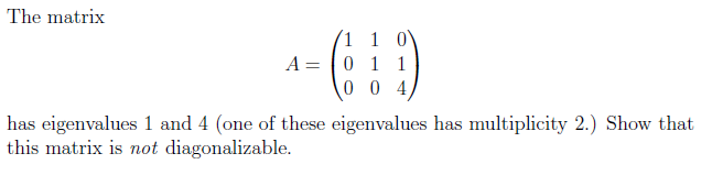
5.2 Diagonalization of Matrices
Unit & Topic Study Guides
Linear Systems and Matrices
Determinants
Vector Spaces
Linear Transformations
Eigenvalues and Eigenvectors
Inner Products and Orthogonality
Intro to Differential Equations
First-Order Differential Equations
Higher-Order Linear Differential Equations
Systems of Differential Equations
Laplace Transforms
Numerical Methods for ODEs
Linear Algebra & DE: Real-World Applications
Diagonalization is a powerful tool in linear algebra, allowing us to simplify complex matrix operations. By transforming a matrix into a diagonal form, we can easily compute powers, exponentials, and solve systems of differential equations.
This process connects to eigenvalues and eigenvectors, as diagonalization requires finding these key components. Understanding diagonalization helps us analyze matrix properties, solve differential equations, and tackle various applications in science and engineering.
Diagonalizability of matrices
Conditions for diagonalizability
- Matrix diagonalizable if it has n linearly independent eigenvectors (n dimension of matrix)
- Algebraic multiplicity counts eigenvalue occurrences as roots of characteristic equation
- Geometric multiplicity measures dimension of eigenspace for each eigenvalue
- Diagonalizability requires geometric multiplicity equal algebraic multiplicity for all distinct eigenvalues
- Matrices with n distinct eigenvalues guaranteed diagonalizable
- Defective matrices (geometric multiplicity < algebraic multiplicity for ≥1 eigenvalue) not diagonalizable
- Diagonalizability test compares sum of eigenspace dimensions to matrix dimension
Analyzing matrix diagonalizability
- Examine eigenvalues and eigenvectors to determine diagonalizability
- Calculate characteristic equation:
- Find eigenvalues by solving characteristic equation
- Compute eigenvectors for each eigenvalue:
- Check linear independence of eigenvectors (Gaussian elimination, determinant method)
- Compare algebraic and geometric multiplicities for each eigenvalue
- Example: 3x3 matrix with eigenvalues 2 (algebraic multiplicity 2) and 5 (algebraic multiplicity 1)
- Diagonalizable if 2 linearly independent eigenvectors for eigenvalue 2 and 1 for eigenvalue 5
- Example: 2x2 rotation matrix always diagonalizable with complex eigenvalues
Eigenvector and diagonal matrices
Constructing eigenvector matrix
- Eigenvector matrix P columns contain linearly independent eigenvectors
- Arrange eigenvectors in same order as corresponding eigenvalues
- Complex eigenvalues may result in complex entries in eigenvector matrix
- Find eigenvectors by solving homogeneous system for each eigenvalue λ
- Normalize eigenvectors to obtain unit vectors (optional but often helpful)
- Ensure number of linearly independent eigenvectors equals geometric multiplicity for each eigenvalue
- Example: For 3x3 matrix A with eigenvalues 2, 2, 5 and corresponding eigenvectors v₁, v₂, v₃:
Forming diagonal matrix
- Diagonal matrix D contains eigenvalues along main diagonal
- Repeat each eigenvalue according to its algebraic multiplicity
- Off-diagonal elements all zero
- Dimension of D matches dimension of original matrix A
- For complex eigenvalues, D may contain complex entries
- Example: 3x3 matrix with eigenvalues 2 (multiplicity 2) and 5 (multiplicity 1):
- Verify diagonalization by checking if
Matrix diagonalization
Diagonalization process
- Express matrix A as product of eigenvector and diagonal matrices:
- P^(-1) columns contain left eigenvectors of A (rows of P^(-1) transposed)
- Transformation effectively changes basis to represent linear transformation as diagonal matrix
- Determinant of A equals product of entries in D after diagonalization
- Trace of A preserved in diagonalization (sum of entries in D)
- For symmetric matrices, P orthogonal matrix simplifies diagonalization to
- Process reveals intrinsic structure of linear transformation represented by matrix A
Applications of diagonalization formula
- Simplify matrix operations using diagonalization
- Compute matrix powers efficiently: (D^n diagonal matrix with entries raised to nth power)
- Calculate matrix exponential: (e^(Dt) diagonal matrix with entries e^(λt))
- Example: Computing A^10 for diagonalizable 3x3 matrix much faster using than direct multiplication
- Example: Solving differential equation using matrix exponential
Applications of diagonalization
Solving systems of differential equations
- Diagonalization simplifies solution of linear differential equations to
- Analyze stability of solutions by examining eigenvalues in diagonal matrix D
- Decouple systems of differential equations allowing independent solution of each equation
- Example: Predator-prey model represented by system of differential equations
- Diagonalization reveals oscillatory behavior or stable equilibrium based on eigenvalues
Matrix analysis and computations
- Efficient computation of matrix powers and exponentials
- Spectral decomposition for symmetric matrices (equivalent to diagonalization)
- Applications in principal component analysis and data reduction techniques
- Markov chain analysis reveals long-term behavior and convergence rates to steady-state distributions
- Example: Google's PageRank algorithm uses eigenvalue analysis to rank web pages
- Example: Image compression using singular value decomposition (related to diagonalization)