2.2 Ordinary least squares (OLS) estimation

Ordinary Least Squares (OLS) is a cornerstone method in econometrics for estimating linear regression models. It finds the best-fitting line by minimizing the sum of squared differences between observed and predicted values, providing insights into relationships between economic variables.

OLS relies on key assumptions like linearity, random sampling, and homoskedasticity. When these assumptions hold, OLS estimators are unbiased, consistent, and efficient. Understanding OLS properties and potential issues is crucial for valid econometric analysis and interpretation.

Definition of OLS

• Ordinary Least Squares (OLS) is a widely used method for estimating the parameters of a linear regression model
• OLS aims to find the line of best fit that minimizes the sum of squared differences between the observed values and the predicted values
• In the context of Introduction to Econometrics, OLS is a fundamental tool for analyzing the relationship between economic variables and making predictions based on the estimated model

Minimizing sum of squared residuals

Top images from around the web for Minimizing sum of squared residuals

• 

  data visualization - Help interpreting Residuals vs Fitted Plots - Cross Validated View original

  Is this image relevant?

• 

  r - 3D plot of the residual sum of squares in linear regression - Stack Overflow View original

  Is this image relevant?

• 

  regression - Residuals follow exactly same pattern as data points - Cross Validated View original

  Is this image relevant?

• 

  data visualization - Help interpreting Residuals vs Fitted Plots - Cross Validated View original

  Is this image relevant?

• 

  r - 3D plot of the residual sum of squares in linear regression - Stack Overflow View original

  Is this image relevant?

1 of 3

Top images from around the web for Minimizing sum of squared residuals

• 

  data visualization - Help interpreting Residuals vs Fitted Plots - Cross Validated View original

  Is this image relevant?

• 

  r - 3D plot of the residual sum of squares in linear regression - Stack Overflow View original

  Is this image relevant?

• 

  regression - Residuals follow exactly same pattern as data points - Cross Validated View original

  Is this image relevant?

• 

  data visualization - Help interpreting Residuals vs Fitted Plots - Cross Validated View original

  Is this image relevant?

• 

  r - 3D plot of the residual sum of squares in linear regression - Stack Overflow View original

  Is this image relevant?

1 of 3

• OLS estimates the regression coefficients by minimizing the sum of squared residuals (SSR)
• Residuals are the differences between the observed values of the dependent variable and the predicted values from the regression line
• By minimizing the SSR, OLS finds the line that best fits the data points, reducing the overall prediction error

Estimating linear regression models

• OLS is commonly used to estimate the parameters of linear regression models
• A linear regression model assumes a linear relationship between the dependent variable and one or more independent variables
• The estimated coefficients from OLS represent the change in the dependent variable associated with a one-unit change in each independent variable, holding other variables constant

Assumptions of OLS

• To obtain reliable and unbiased estimates, OLS relies on several key assumptions about the data and the model
• Violating these assumptions can lead to biased or inefficient estimates, affecting the validity of the regression results
• It is crucial to assess whether these assumptions hold in practice and take appropriate measures if they are violated

Linearity in parameters

• OLS assumes that the relationship between the dependent variable and the independent variables is linear in parameters
• This means that the regression coefficients enter the model linearly, even if the independent variables themselves are non-linear (quadratic, logarithmic, etc.)
• Departures from linearity can be addressed by transforming variables or using non-linear regression techniques

Random sampling

• OLS assumes that the data is obtained through random sampling from the population of interest
• Random sampling ensures that the observations are independent and identically distributed (i.i.d.)
• Non-random sampling or selection bias can lead to biased estimates and invalid inferences

No perfect collinearity

• OLS assumes that there is no perfect collinearity among the independent variables
• Perfect collinearity occurs when one independent variable is an exact linear combination of other independent variables
• In the presence of perfect collinearity, OLS cannot uniquely estimate the coefficients, leading to unreliable results
• Near-perfect collinearity (high correlation) can also cause issues, such as inflated standard errors and unstable coefficient estimates

Zero conditional mean

• OLS assumes that the error term has a zero conditional mean given the values of the independent variables
• Mathematically, $E[u|X] = 0$, where $u$ is the error term and $X$ represents the independent variables
• This assumption implies that the independent variables are exogenous and uncorrelated with the error term
• Violation of this assumption, known as endogeneity, can lead to biased and inconsistent estimates

Homoskedasticity

• OLS assumes that the error term has constant variance across all levels of the independent variables
• Homoskedasticity implies that the spread of the residuals is constant, regardless of the values of the independent variables
• Violation of this assumption, known as heteroskedasticity, can lead to inefficient estimates and invalid standard errors
• Heteroskedasticity can be detected using tests like the Breusch-Pagan test or White's test, and can be addressed using robust standard errors or weighted least squares

Properties of OLS estimators

• Under the assumptions of OLS, the estimated coefficients possess desirable statistical properties that make them reliable and efficient
• These properties are crucial for making valid inferences and predictions based on the estimated model
• Understanding these properties helps in assessing the quality and reliability of the OLS estimates

Unbiasedness

• OLS estimators are unbiased, meaning that the expected value of the estimated coefficients is equal to the true population parameters
• Mathematically, $E[\hat{\beta}] = \beta$, where $\hat{\beta}$ is the OLS estimator and $\beta$ is the true parameter
• Unbiasedness ensures that, on average, the OLS estimates are centered around the true values
• Unbiasedness is a desirable property as it indicates that the estimators are accurate on average

Consistency

• OLS estimators are consistent, meaning that as the sample size increases, the estimates converge in probability to the true population parameters
• Mathematically, $\hat{\beta} \xrightarrow{p} \beta$ as $n \rightarrow \infty$, where $n$ is the sample size
• Consistency implies that with a large enough sample, the OLS estimates become more precise and closer to the true values
• Consistency is important for making reliable inferences and predictions, especially when working with large datasets

Efficiency

• OLS estimators are efficient among the class of linear unbiased estimators
• Efficiency means that OLS estimators have the smallest variance among all unbiased estimators
• This property is known as the Best Linear Unbiased Estimator (BLUE) property, which is formally stated in the ###Gauss-Markov_Theorem_0###
• Efficient estimators provide the most precise estimates, leading to narrower confidence intervals and more powerful hypothesis tests

Gauss-Markov theorem

• The Gauss-Markov theorem is a fundamental result in econometrics that establishes the optimality of OLS estimators under certain assumptions
• It states that, under the assumptions of linearity, random sampling, no perfect collinearity, zero conditional mean, and homoskedasticity, OLS estimators are the Best Linear Unbiased Estimators (BLUE)
• The theorem provides a strong justification for using OLS in linear regression analysis

Best linear unbiased estimator (BLUE)

• BLUE is a desirable property of an estimator that combines unbiasedness and efficiency
• An estimator is BLUE if it is linear in the dependent variable, unbiased, and has the smallest variance among all linear unbiased estimators
• OLS estimators satisfy the BLUE property under the Gauss-Markov assumptions, making them optimal in the class of linear unbiased estimators

OLS vs other estimators

• While OLS is BLUE under the Gauss-Markov assumptions, there may be situations where other estimators are preferred
• For example, if the assumptions of homoskedasticity or no perfect collinearity are violated, OLS may not be the most efficient estimator
• In such cases, alternative estimators like Generalized Least Squares (GLS) or robust estimators may be more appropriate
• However, OLS remains a widely used and reliable estimator in many practical applications due to its simplicity and desirable properties

Estimating OLS coefficients

• Estimating the coefficients of an OLS regression model involves finding the values of the slope and intercept that minimize the sum of squared residuals
• The estimation process can be done using various methods, including the formulas for slope and intercept or matrix notation
• Understanding the estimation process is essential for interpreting the results and assessing the model's performance

Formulas for slope and intercept

• For a simple linear regression model with one independent variable, the OLS estimates of the slope ($\hat{\beta}_1$) and intercept ($\hat{\beta}_0$) can be calculated using the following formulas:
  • Slope: $\hat{\beta}_1 = \frac{\sum_{i=1}^{n}(x_i - \bar{x})(y_i - \bar{y})}{\sum_{i=1}^{n}(x_i - \bar{x})^2}$
  • Intercept: $\hat{\beta}_0 = \bar{y} - \hat{\beta}_1\bar{x}$
• Here, $x_i$ and $y_i$ are the values of the independent and dependent variables for observation $i$, and $\bar{x}$ and $\bar{y}$ are the sample means of $x$ and $y$, respectively
• These formulas provide a straightforward way to calculate the OLS estimates in a simple linear regression setting

Matrix notation

• For multiple linear regression models with more than one independent variable, matrix notation provides a compact and efficient way to estimate the OLS coefficients
• In matrix notation, the regression model is expressed as $y = X\beta + u$, where:
  • $y$ is an $n \times 1$ vector of the dependent variable
  • $X$ is an $n \times k$ matrix of independent variables (including a column of ones for the intercept)
  • $\beta$ is a $k \times 1$ vector of coefficients
  • $u$ is an $n \times 1$ vector of error terms
• The OLS estimator of $\beta$ is given by: $\hat{\beta} = (X'X)^{-1}X'y$
• Matrix notation simplifies the calculations and allows for efficient estimation of the coefficients using statistical software packages

Interpreting OLS results

• After estimating an OLS regression model, it is crucial to interpret the results correctly to draw meaningful conclusions and make informed decisions
• Interpreting OLS results involves examining the coefficient estimates, standard errors, confidence intervals, and hypothesis tests
• These components provide insights into the relationship between the variables and the statistical significance of the estimates

Coefficient estimates

• The estimated coefficients from an OLS regression represent the change in the dependent variable associated with a one-unit change in each independent variable, holding other variables constant
• For example, if the coefficient estimate for an independent variable is 0.5, it means that a one-unit increase in that variable is associated with a 0.5-unit increase in the dependent variable, ceteris paribus
• The interpretation of the coefficients depends on the scale and units of the variables involved
• It is important to consider the practical and economic significance of the coefficient estimates, not just their statistical significance

Standard errors

• Standard errors provide a measure of the uncertainty associated with the coefficient estimates
• They indicate the average amount by which the coefficient estimates would vary if the regression were repeated many times using different samples from the same population
• Smaller standard errors suggest more precise estimates and greater confidence in the results
• Standard errors are used to construct confidence intervals and perform hypothesis tests

Confidence intervals

• Confidence intervals provide a range of plausible values for the true population parameters based on the sample estimates
• A 95% confidence interval, for example, is constructed as the coefficient estimate ± 1.96 × standard error
• The interpretation is that if the sampling process were repeated many times, 95% of the resulting confidence intervals would contain the true parameter value
• Wider confidence intervals indicate greater uncertainty in the estimates, while narrower intervals suggest more precise estimates

Hypothesis testing

• Hypothesis testing allows researchers to assess the statistical significance of the coefficient estimates
• The null hypothesis typically states that the coefficient is equal to zero, implying no relationship between the independent variable and the dependent variable
• The alternative hypothesis suggests that the coefficient is different from zero
• The test statistic, usually a t-statistic or an F-statistic, is calculated and compared to a critical value or a p-value to make a decision about rejecting or failing to reject the null hypothesis
• A small p-value (typically less than 0.05) indicates strong evidence against the null hypothesis, suggesting that the coefficient is statistically significant

Goodness of fit

• Goodness of fit measures assess how well the estimated OLS model fits the observed data
• These measures provide information about the explanatory power of the model and the proportion of the variation in the dependent variable that is explained by the independent variables
• The most commonly used goodness of fit measures in OLS regression are R-squared and adjusted R-squared

R-squared

• R-squared, also known as the coefficient of determination, measures the proportion of the variation in the dependent variable that is explained by the independent variables in the model
• R-squared ranges from 0 to 1, with higher values indicating a better fit
• An R-squared of 0.7, for example, means that 70% of the variation in the dependent variable is explained by the independent variables in the model
• R-squared is calculated as the ratio of the explained sum of squares (ESS) to the total sum of squares (TSS): $R^2 = \frac{ESS}{TSS} = 1 - \frac{SSR}{TSS}$
• While R-squared provides a measure of the model's explanatory power, it has some limitations, such as increasing with the addition of more independent variables, even if they are not relevant

Adjusted R-squared

• Adjusted R-squared is a modified version of R-squared that accounts for the number of independent variables in the model
• Unlike R-squared, adjusted R-squared penalizes the inclusion of irrelevant variables, making it a more reliable measure of goodness of fit
• Adjusted R-squared is calculated as: $\bar{R}^2 = 1 - \frac{(1-R^2)(n-1)}{n-k-1}$, where $n$ is the sample size and $k$ is the number of independent variables
• Adjusted R-squared is always lower than or equal to R-squared, and it can decrease with the addition of irrelevant variables
• When comparing models with different numbers of independent variables, adjusted R-squared is preferred over R-squared

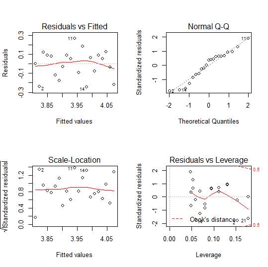
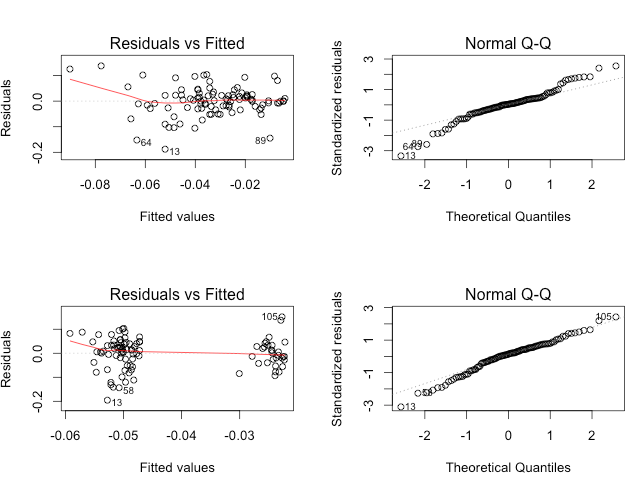
Potential issues with OLS

• While OLS is a powerful and widely used estimation method, it is not without its limitations and potential issues
• Violating the assumptions of OLS can lead to biased, inconsistent, or inefficient estimates, affecting the reliability of the results
• It is essential to be aware of these potential issues and take appropriate measures to address them

Omitted variable bias

• Omitted variable bias occurs when a relevant variable is excluded from the regression model
• If the omitted variable is correlated with both the dependent variable and one or more of the included independent variables, the estimated coefficients of the included variables will be biased
• Omitted variable bias can lead to incorrect conclusions about the relationship between the variables and the magnitude of the effects
• To mitigate omitted variable bias, researchers should carefully consider the theoretical foundations of the model and include all relevant variables based on prior knowledge and economic theory

Measurement error

• Measurement error refers to the difference between the true value of a variable and its observed or recorded value
• Measurement error in the independent variables can lead to biased and inconsistent estimates, a problem known as errors-in-variables bias
• Classical measurement error, where the errors are uncorrelated with the true values and other variables, tends to bias the coefficient estimates towards zero (attenuation bias)
• Strategies to address measurement error include using instrumental variables, obtaining more accurate data, or using specialized estimation techniques like errors-in-variables regression

Endogeneity

• Endogeneity occurs when an independent variable is correlated with the error term, violating the zero conditional mean assumption of OLS
• Endogeneity can arise due to omitted variables, measurement error, simultaneous causality, or sample selection bias
• In the presence of endogeneity, OLS estimates will be biased and inconsistent, leading to incorrect inferences about the relationship between the variables
• Addressing endogeneity often requires the use of instrumental variables, which are variables that are correlated with the endogenous independent variable but uncorrelated with the error term

Heteroskedasticity

• Heteroskedasticity refers to the violation of the constant variance assumption of OLS, where the variance of the error term varies across different levels of the independent variables
• In the presence of heteroskedasticity, OLS estimates remain unbiased and consistent but are no longer efficient, leading to invalid standard errors and hypothesis tests
• Heteroskedasticity can be detected using tests like the Breusch-Pagan test or White's test
• To address heteroskedasticity, researchers can use robust standard errors, which provide valid inference in the presence of heteroskedasticity, or employ weighted least squares (WLS) estimation

Autocorrelation

• Autocorrelation, also known as serial correlation, occurs when the error terms are correlated across observations, typically in time series data
• Autocorrelation violates the assumption of independent and identically distributed (i.i.d.) errors, leading to inefficient estimates and invalid standard errors
• Positive autocorrelation, where errors are positively correlated over time, is more common in practice
• Autocorrelation can be detected using tests like the Durbin-Watson test or the Breusch-Godfrey test
• To address autocorrelation, researchers can use methods like generalized least squares (GLS), autoregressive models (e.g., AR(1) correction), or Newey-West standard errors

Remedies for OLS issues

• When the assumptions of OLS are violated, there are several remedies that can be employed to address the issues and obtain more reliable estimates
• These remedies involve modifying the regression model, using alternative estimation techniques, or adjusting the standard errors
• The choice of the appropriate remedy depends on the specific issue and the nature of the data

Adding control variables

• One way to address omitted variable bias is by adding relevant control variables to the regression model
• Control variables are factors that are believed to influence the dependent variable but are not the primary focus of the analysis
• By including control variables, researchers can account for potential confounding factors and obtain more accurate estimates of the relationship between the main independent variables and the dependent variable
• The selection of control variables should be guided by economic theory and prior knowledge about the relationships among the variables

Instrumental variables

• Instrumental variables (IV) estimation is a technique used to address endogeneity and obtain consistent estimates in the presence of correlated errors
• An instrumental variable is a variable that is correlated with the endogen