3.4 Inverse Laplace Transforms

Inverse Laplace transforms are crucial for converting frequency-domain functions back to the time domain. This process helps engineers analyze system behavior and responses to different inputs. It's a key tool for understanding dynamic systems.

Mastering inverse Laplace transforms allows you to find time-domain solutions to differential equations and analyze transfer functions. This skill is essential for predicting system outputs, stability, and transient responses in various engineering applications.

Partial fraction decomposition for Laplace transforms

Decomposing rational functions

Top images from around the web for Decomposing rational functions

• 

  A Partial fraction expansion questions about Laplace transform - Mathematics Stack Exchange View original

  Is this image relevant?

• 

  How do you find the Inverse Laplace transformation for a product of $2$ functions? - Mathematics ... View original

  Is this image relevant?

• 

  differential equations - How to solve laplace inverse using convolution - Mathematics Stack Exchange View original

  Is this image relevant?

• 

  A Partial fraction expansion questions about Laplace transform - Mathematics Stack Exchange View original

  Is this image relevant?

• 

  How do you find the Inverse Laplace transformation for a product of $2$ functions? - Mathematics ... View original

  Is this image relevant?

1 of 3

Top images from around the web for Decomposing rational functions

• 

  A Partial fraction expansion questions about Laplace transform - Mathematics Stack Exchange View original

  Is this image relevant?

• 

  How do you find the Inverse Laplace transformation for a product of $2$ functions? - Mathematics ... View original

  Is this image relevant?

• 

  differential equations - How to solve laplace inverse using convolution - Mathematics Stack Exchange View original

  Is this image relevant?

• 

  A Partial fraction expansion questions about Laplace transform - Mathematics Stack Exchange View original

  Is this image relevant?

• 

  How do you find the Inverse Laplace transformation for a product of $2$ functions? - Mathematics ... View original

  Is this image relevant?

1 of 3

• Partial fraction expansion decomposes rational functions into a sum of simpler rational functions
• Enables the use of a Laplace transform table to find the inverse transform
• Proper rational functions have the degree of the numerator less than the degree of the denominator
  • Performed by factoring the denominator and setting up a system of linear equations to solve for coefficients
• Improper rational functions have the degree of the numerator greater than or equal to the degree of the denominator
  • Must first be divided using long division to separate the polynomial and proper rational function parts
  • Partial fraction expansion is then applied to the proper rational function part

Handling special cases in partial fraction decomposition

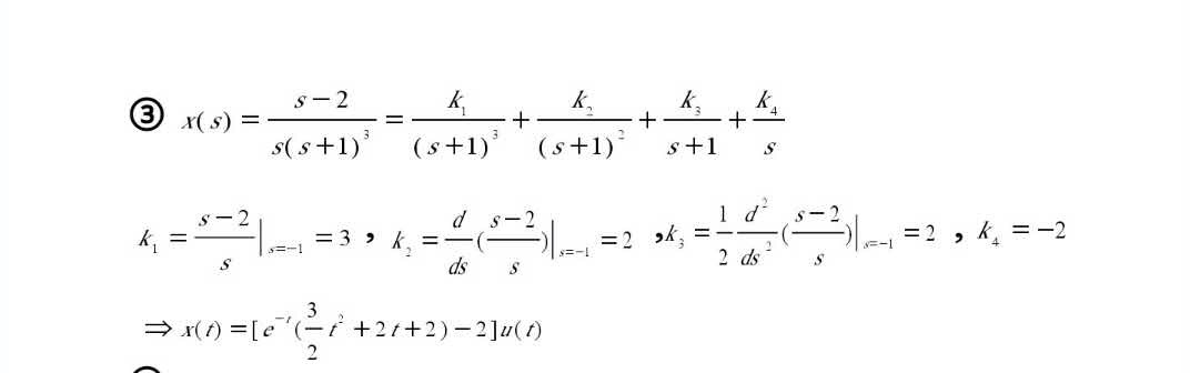
• When the denominator contains repeated linear factors, the partial fraction expansion includes terms with powers of the linear factors in the denominators
  • Example: $\frac{1}{(s+2)^2(s-1)}$ would have terms like $\frac{A}{s+2}$, $\frac{B}{(s+2)^2}$, and $\frac{C}{s-1}$
• For quadratic factors in the denominator that cannot be factored into real linear terms, the partial fraction expansion includes terms with the quadratic factor in the denominator and linear terms in the numerator
  • Example: $\frac{1}{s^2+4s+5}$ would have a term like $\frac{As+B}{s^2+4s+5}$
• Proper rational functions with irreducible quadratic factors in the denominator will have linear terms in the numerator for each quadratic factor
• Improper rational functions may require a combination of long division and partial fraction expansion to fully decompose the function

Inverse Laplace transforms using tables

Using a table of common transforms

• The inverse Laplace transform converts a function from the s-domain (frequency domain) back to the time domain
• Reverses the Laplace transform process
• A table of common Laplace transforms and their corresponding inverse Laplace transforms is used to find the time-domain function
• The table includes transforms for basic functions (exponential, trigonometric, polynomial) and more complex functions (unit step function, Dirac delta function)

Applying properties of inverse Laplace transforms

• Linearity properties allow for the inverse transform of a sum of functions to be the sum of the inverse transforms of each function
  • Example: $\mathcal{L}^{-1}\{F(s)+G(s)\}=\mathcal{L}^{-1}\{F(s)\}+\mathcal{L}^{-1}\{G(s)\}$
• The time-shift property states that multiplying the s-domain function by $e^{-as}$, where $a$ is a constant, results in a time-shift of the original time-domain function by $a$ units
  • Example: $\mathcal{L}^{-1}\{e^{-as}F(s)\}=f(t-a)u(t-a)$, where $f(t)=\mathcal{L}^{-1}\{F(s)\}$ and $u(t)$ is the unit step function
• The scaling property allows for the inverse Laplace transform of a scaled function to be determined by scaling the time-domain function
  • Example: $\mathcal{L}^{-1}\{F(as)\}=\frac{1}{a}f(\frac{t}{a})$, where $f(t)=\mathcal{L}^{-1}\{F(s)\}$

Time-domain response from transfer functions

Finding the time-domain response

• The transfer function of a system is the ratio of the Laplace transform of the output to the Laplace transform of the input, assuming zero initial conditions
• To find the time-domain response, multiply the transfer function by the Laplace transform of the input function
• Apply the inverse Laplace transform to the resulting product
• For rational transfer functions, partial fraction expansion is often necessary to decompose the function into a form suitable for finding the inverse Laplace transform using a table

Using alternative methods for time-domain response

• The initial value theorem determines the initial value of the time-domain response without explicitly finding the inverse Laplace transform
  • Example: $\lim_{t\to 0}f(t)=\lim_{s\to\infty}sF(s)$, where $f(t)$ is the time-domain function and $F(s)$ is its Laplace transform
• The final value theorem determines the steady-state value of the time-domain response without explicitly finding the inverse Laplace transform
  • Example: $\lim_{t\to\infty}f(t)=\lim_{s\to 0}sF(s)$, assuming the limit exists
• The convolution integral finds the time-domain response by convolving the input function with the inverse Laplace transform of the transfer function (impulse response)
  • Example: $y(t)=\int_{0}^{t}h(t-\tau)x(\tau)d\tau$, where $y(t)$ is the output, $x(t)$ is the input, and $h(t)$ is the impulse response

Time-domain behavior from inverse Laplace transforms

Identifying key characteristics

• The inverse Laplace transform of a system's transfer function yields the time-domain impulse response
• Characterizes the system's behavior when subjected to an impulse input
• Key characteristics include stability, rise time, settling time, and steady-state value
  • Stable systems have an impulse response that decays to zero as time approaches infinity
  • Unstable systems have an impulse response that grows without bound
• Rise time is the time required for the response to rise from a small percentage (10%) to a large percentage (90%) of its final value
  • Indicates the system's speed of response
• Settling time is the time required for the response to settle within a certain percentage (2%) of its final value
  • Indicates the time needed to reach steady-state

Analyzing oscillatory behavior and steady-state values

• Oscillatory behavior in the time-domain response is identified by the presence of sinusoidal terms in the inverse Laplace transform
• The frequency of oscillation is determined by the coefficients of the imaginary components
  • Example: $\mathcal{L}^{-1}\{\frac{1}{s^2+\omega^2}\}=\frac{1}{\omega}\sin(\omega t)$, where $\omega$ is the frequency of oscillation
• The steady-state value of the time-domain response can be determined using the final value theorem
  • States that the steady-state value is equal to the limit of $s$ times the transfer function as $s$ approaches zero, assuming the limit exists
  • Example: $\lim_{t\to\infty}y(t)=\lim_{s\to 0}sY(s)$, where $y(t)$ is the time-domain output and $Y(s)$ is its Laplace transform
• Damping in the system affects the oscillatory behavior and the rate at which the response settles to its steady-state value
  • Overdamped systems have no oscillations and settle slowly
  • Underdamped systems have oscillations that decay over time
  • Critically damped systems have no oscillations and settle in the shortest possible time without overshoot