Amdahl's Law predicts how much faster a program can run when you spread its work across multiple processors. It reveals a fundamental constraint: the serial (non-parallelizable) portion of a program puts a hard ceiling on speedup, no matter how many processors you throw at it. Understanding this law helps you decide whether adding processors is worthwhile or whether your time is better spent optimizing the serial code.
Amdahl's Law in Parallel Computing
Concept and Implications
Amdahl's Law gives you a formula for the theoretical maximum speedup of a program running on multiple processors. The core idea is that every program has two parts: a parallelizable fraction (work that can be split across processors) and a serial fraction (work that must run on a single processor, one step at a time).
The serial fraction is the bottleneck. As you add more processors, the parallel portion gets faster, but the serial portion stays the same. This means speedup hits a wall determined entirely by how large the serial fraction is.
- If 10% of a program is serial, the maximum theoretical speedup is , even with infinite processors.
- If 50% is serial, the ceiling drops to just .
- Diminishing returns kick in quickly: each additional processor contributes less speedup than the one before it.
This has a practical consequence that's easy to overlook. Shrinking the serial portion often matters more than adding processors. For example, reducing the serial fraction from 20% to 10% doubles your maximum theoretical speedup (from to ).
Speedup Calculation Formula
The formula is:
where:
- = the fraction of the program that can be parallelized
- = the serial fraction
- = the number of processors
Example: If 75% of a program is parallelizable () and you run it on 4 processors:
Notice that even though you quadrupled the processors, you didn't get anywhere close to a speedup. That gap is entirely due to the 25% serial portion.
Theoretical Speedup Calculation

Steps to Calculate Speedup
-
Identify the parallelizable fraction (). The serial fraction is .
-
Determine the number of processors () you'll use.
-
Plug into the formula:
-
Compute the result by evaluating the denominator first, then dividing 1 by it.
Worked example: A program has 60% parallelizable code () and runs on 8 processors.
- Serial fraction:
- Parallel portion per processor:
- Denominator:
- Speedup:
Even with 8 processors, the 40% serial fraction keeps speedup just above .
Impact of Parallelizable Fraction and Processor Count
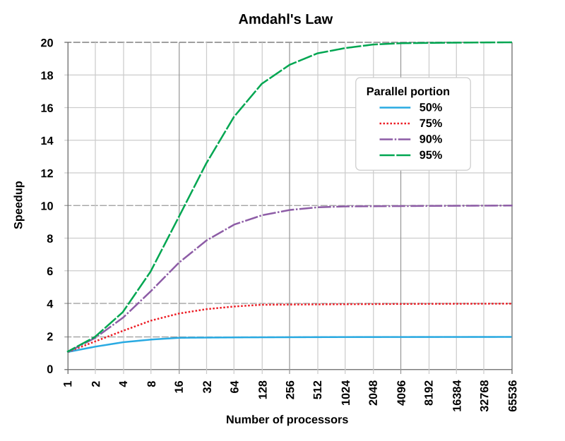
The parallelizable fraction has a much larger effect on speedup than the processor count . Here's a comparison:
| (ceiling) | |||
|---|---|---|---|
| 0.50 | 1.60 | 1.88 | 2.00 |
| 0.80 | 2.50 | 3.33 | 5.00 |
| 0.90 | 3.08 | 5.93 | 10.00 |
| 0.95 | 3.48 | 7.80 | 20.00 |
Two things stand out in this table. First, going from to at 16 processors triples your speedup. Second, going from 4 to 16 processors at only gains you about more speedup despite quadrupling hardware. The returns from adding processors diminish fast, especially when the serial portion is large.
Amdahl's Law Limitations
Assumptions and Real-World Constraints
Amdahl's Law is a useful model, but it makes several simplifying assumptions that don't always hold in practice.
- Fixed problem size. The law assumes you're solving the same-sized problem with more processors. In many real applications, you scale the problem up as you add processors (called weak scaling). Gustafson's Law addresses this alternative scenario and often gives a more optimistic view of parallel speedup.
- No parallelization overhead. The formula ignores the cost of coordinating processors: communication, synchronization, thread creation, and data sharing. These overheads grow as you add processors, so actual speedup is typically lower than what Amdahl's Law predicts.
- Perfect load balancing. The law assumes work divides evenly across all processors. In practice, dependencies between tasks or uneven data partitions can leave some processors idle while others are still working, which wastes resources and reduces speedup.
Other Factors Affecting Parallel Performance
Several real-world factors fall outside the scope of Amdahl's Law:
- Memory hierarchy and data locality. When processors need to access shared memory or data stored on remote nodes, latency and bandwidth limitations can slow things down significantly. Keeping data close to the processor that needs it (locality optimization) is critical.
- Resource contention. Parallel systems often run multiple programs at once. Processors competing for shared cache, memory bandwidth, or interconnect capacity can degrade each program's performance.
- The serial fraction isn't always fixed. Some code that looks serial can sometimes be restructured. Techniques like pipelining, speculative execution, or algorithmic redesign can shrink the serial portion, pushing the speedup ceiling higher than the original analysis suggested.
Speedup Analysis Techniques
Measuring and Comparing Speedup
To evaluate a real parallel program, you compare measured performance against the theoretical prediction.
- Measure sequential execution time () by running the program on a single processor.
- Measure parallel execution time () on your target number of processors.
- Calculate actual speedup:
For example, if the sequential run takes 100 seconds and the 4-processor run takes 30 seconds, the actual speedup is .
Now compare to the theoretical from Amdahl's Law. If actual speedup falls well below the theoretical value, something is eating into your performance: overhead, load imbalance, or memory bottlenecks are the usual suspects.
Profiling and Optimization Strategies
Scalability analysis helps you understand how your program behaves as you change resources:
- Strong scaling: Keep the problem size fixed and increase the number of processors. You're testing how well the program parallelizes at that size.
- Weak scaling: Increase both the problem size and processor count proportionally. You're testing whether the program maintains performance as the workload grows.
Profiling tools like Intel VTune, GNU gprof, or OpenMP profiling interfaces help you pinpoint where time is actually being spent. Focus your optimization on the sections that consume the most time, since small improvements to hot spots yield the biggest gains.
Parallelization strategies to consider:
- Data parallelism: Partition the data and apply the same operation to each partition simultaneously. Works well when the same computation repeats across a large dataset.
- Task parallelism: Distribute independent tasks across processors. Best when the program has many distinct operations that don't depend on each other.
- Pipeline parallelism: Split computation into stages and feed data through them concurrently, similar to an assembly line. Useful when processing a stream of inputs through multiple steps.
Choosing the right strategy depends on the structure of your problem and the architecture you're targeting. Often, the best approach involves combining strategies for different parts of the program.