Types of Climate Models
Climate models are digital tools that simulate Earth's climate system. They range from simple calculations of energy in vs. energy out, all the way to massive simulations that model the atmosphere, oceans, ice sheets, and living ecosystems together. Understanding the different types of models, and how they've improved over time, is central to understanding how scientists forecast climate change.
Types of climate models
Energy Balance Models (EBMs) are the simplest type. They focus on one core question: how much energy does Earth receive from the Sun, and how much does it radiate back to space? EBMs treat the Earth as a single point or a small number of latitude bands, so they don't represent winds, ocean currents, or other dynamic processes. Despite that simplicity, they're genuinely useful for exploring basic climate feedbacks like the greenhouse effect and albedo (how reflective Earth's surface is).
Earth System Models of Intermediate Complexity (EMICs) sit in the middle. They include some atmospheric and ocean dynamics but use coarser spatial resolution or simplified physics compared to full-scale models. Their real strength is efficiency: because they run faster, they're used for simulations spanning thousands to millions of years. That makes them ideal for studying slow processes like ice sheet growth or long-term carbon cycle feedbacks. Examples include UVic ESCM and CLIMBER.
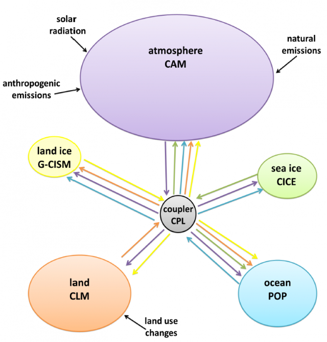
General Circulation Models (GCMs) are the most comprehensive type. They divide the atmosphere and oceans into a three-dimensional grid and solve equations for fluid dynamics, thermodynamics, and radiative transfer within each grid cell. GCMs come in two main flavors:
- Coupled Atmosphere-Ocean GCMs (AOGCMs) simulate the interactions between the atmosphere and oceans together, capturing processes like heat exchange at the sea surface.
- Earth System Models (ESMs) build on AOGCMs by adding components like the carbon cycle, dynamic vegetation, and ice sheets. This makes them the most complete representation of the climate system available.
Examples of GCMs/ESMs include CESM, HadGEM, and IPSL-CM.

Development of climate models
Climate models have improved dramatically since the 1970s, driven by several key factors:
- New scientific understanding. As researchers learn more about climate processes, models get updated. For instance, the way models represent cloud behavior (microphysics, convection), aerosol effects (both direct scattering and indirect effects on clouds), and carbon uptake by land and oceans has all improved significantly over the decades.
- Increased spatial resolution. Greater computing power allows finer grid cells. Typical resolutions have gone from roughly 500 km in the 1970s to around 25 km today. Finer grids mean models can better capture features like mountain ranges, coastlines, and extreme weather events such as tropical cyclones and heavy precipitation.
- Addition of new components. Early models only simulated the atmosphere. Over time, oceans, sea ice, land surfaces, dynamic vegetation, ice sheets, and atmospheric chemistry (ozone, methane) have all been added. Each new component lets the model capture feedbacks it previously had to ignore.
- Improved parameterizations. Processes too small for the grid (like individual cloud droplets forming) get represented through simplified equations called parameterizations. As observational data improves, so do these approximations. More on this below.
- Model intercomparison projects. The Coupled Model Intercomparison Project (CMIP) coordinates experiments across dozens of modeling groups worldwide. By running the same scenarios in different models, CMIP reveals where models agree (building confidence) and where they diverge (highlighting areas that need work). CMIP results feed directly into IPCC assessment reports.
Parameterization in climate modeling
Some physical processes happen at scales much smaller than a model's grid cell. Cloud formation, boundary layer turbulence, and cumulus convection are all examples. A grid cell might be 25 km across, but a single thunderstorm updraft is only a few kilometers wide. The model can't simulate that updraft directly, so it needs another approach.
Parameterizations are simplified equations that estimate the effects of these subgrid-scale processes on the larger climate. For example, a cloud parameterization might estimate what fraction of a grid cell is covered by clouds and what their radiative properties are, based on the cell's humidity and temperature.
The choice of parameterization scheme matters a lot. Different schemes can produce noticeably different results, especially for climate sensitivity (how much warming you get from a given increase in ). For deep convection alone, models might use the Arakawa-Schubert scheme, the Kain-Fritsch scheme, or others, and each handles the physics slightly differently. This is one of the main reasons different climate models can give different projections even when given the same inputs.
Improving parameterizations is an active area of research. High-resolution observations from satellites and field campaigns provide better data to test against, and newer approaches like machine learning and stochastic (randomized) parameterizations are being explored to better capture the inherent variability of small-scale processes.
Validation of climate models
Building a model is only half the job. Scientists also need to check whether the model actually reproduces observed climate behavior. This process is called validation (or evaluation).
Validation typically works by running the model over a historical period and comparing its output to real-world data:
- Instrumental records of temperature, precipitation, and other variables
- Satellite observations of radiation budgets, sea surface temperatures, and ice extent
- Proxy data (ice cores, tree rings) for periods before modern instruments existed
This comparison reveals where models perform well and where they struggle. Models generally do a strong job simulating large-scale patterns and long-term global temperature trends. They tend to have more difficulty with regional precipitation patterns and the frequency of extreme events.
Specific techniques for evaluation include:
- Statistical measures like correlation (R), root-mean-square error (RMSE), and bias, which quantify how closely model output matches observations
- Visual comparison of spatial maps and time series to check whether the model captures the right patterns and trends
- Detection and attribution studies that test whether a model can reproduce observed climate changes only when human forcings (greenhouse gases, aerosols) are included, not from natural variability alone
These evaluations guide future development. If models consistently struggle to simulate El Niño events accurately, for example, that tells developers to focus on improving ocean-atmosphere coupling. As each new generation of models arrives (e.g., CMIP6 replacing CMIP5), it gets tested against an expanding set of observations and forcing scenarios, steadily building confidence in climate projections.