1.3 Degrees of freedom

Degrees of freedom overview

Degrees of freedom (DOF) describes the number of independent ways a robotic system can move. If you can count how many separate motions a robot needs to fully position and orient itself, you've found its DOF. This concept sits at the heart of robot design because it determines what a robot can and can't do.

Definition of DOF

DOF is the minimum number of independent variables needed to completely describe the position and orientation of a robot in space. Each DOF corresponds to one independent motion: either sliding along an axis (translation) or spinning around an axis (rotation).

• A door hinge has 1 DOF: it can only rotate around one axis.
• Your shoulder has roughly 3 DOF: it can rotate in three different directions.
• The total DOF of a robot is the sum of the DOF contributed by all its joints.

Importance in robotics

DOF directly shapes what tasks a robot can handle. More DOF generally means more versatility, since the robot can reach more positions and orientations. But there's a tradeoff: every added DOF increases the complexity of the mechanical design, the control software, and the motion planning.

A good robot design picks just enough DOF for the job. A simple pick-and-place robot on an assembly line might only need 3-4 DOF, while a robot arm performing surgery might need 7 or more.

Types of DOF

DOF falls into two categories: translational (linear movement) and rotational (angular movement). A rigid body floating freely in 3D space has 6 total DOF: 3 translational and 3 rotational.

Translational DOF

Translational DOF is the ability to move in a straight line along an axis. In a standard Cartesian coordinate system, that means movement along x, y, or z.

• A prismatic joint (also called a sliding joint) provides 1 translational DOF. Think of a drawer sliding in and out, or a hydraulic cylinder extending and retracting.
• Cartesian robots and gantry systems rely heavily on prismatic joints to move along straight paths.

Rotational DOF

Rotational DOF is the ability to spin around an axis. The three rotational axes are commonly called roll (spinning like a log), pitch (tilting forward/backward like nodding), and yaw (turning left/right like shaking your head "no").

• A revolute joint (also called a hinge joint) provides 1 rotational DOF. A servo motor spinning a robot arm segment is a classic example.
• Revolute joints are the most common joint type in robotic manipulators because they enable articulated, arm-like motion.

Calculating DOF

To figure out how many independent motions a robot can perform, you need a systematic method. The standard approach is Gruebler's equation (sometimes called the Kutzbach-Gruebler criterion), which accounts for the number of links, joints, and constraints.

Gruebler's equation

The general form for spatial (3D) mechanisms is:

$DOF = 6(n - 1) - 5j_1 - 4j_2 - 3j_3 - 2j_4 - j_5$

Where:

• $n$ = number of links, including the fixed base
• $j_1$ = number of 1-DOF joints (prismatic or revolute)
• $j_2$ = number of 2-DOF joints (e.g., universal joints)
• $j_3$ = number of 3-DOF joints (e.g., spherical/ball joints)
• $j_4, j_5$ = joints with 4 or 5 DOF (less common)

The logic: a free-floating body in 3D has 6 DOF. Each link added to the system brings 6 potential DOF, but the ground link is fixed (hence $n - 1$). Each joint then removes DOF by constraining relative motion between links. A 1-DOF joint removes 5 of the 6 possible relative motions, a 2-DOF joint removes 4, and so on.

Examples of DOF calculation

Planar 3R arm (3 revolute joints, 4 links including the base):

$DOF = 6(4 - 1) - 5(3) = 18 - 15 = 3$

Three revolute joints give 3 DOF, which makes sense: each joint contributes one independent rotation.

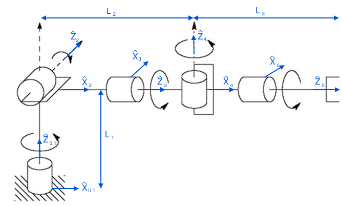
Spatial 6R arm (6 revolute joints, 7 links including the base):

$DOF = 6(7 - 1) - 5(6) = 36 - 30 = 6$

This is the classic 6-DOF industrial robot arm, with enough freedom for full position and orientation control of the end-effector.

Stewart platform (6 prismatic actuators connecting a base to a moving platform, with spherical and universal joints at the connections; 14 links total including the base and platform):

The Stewart platform achieves 6 DOF for the moving platform. The exact Gruebler calculation requires careful counting of all joints and links in the closed-loop structure, but the result is 6 DOF: 3 translational and 3 rotational.

DOF in robotic joints

Joints are what give a robot its DOF. Each joint type allows a specific kind and number of independent motions between the links it connects.

Prismatic joints

• Allow translation along a single axis (1 DOF)
• The connected links slide relative to each other
• Implemented with hydraulic cylinders, lead screws, or linear bearings
• Common in Cartesian robots and gantry systems

Revolute joints

• Allow rotation about a single axis (1 DOF)
• The connected links pivot relative to each other
• Implemented with servo motors, stepper motors, or pin hinges
• The most widely used joint type in robotic arms

Spherical joints

• Allow rotation about three orthogonal axes (3 DOF)
• Think of a ball sitting in a socket: it can roll, pitch, and yaw
• Implemented as ball joints or combinations of universal joints
• Found in robotic wrists, parallel manipulators, and mechanisms that need multi-axis rotation at a single point

DOF vs mobility

DOF and mobility are related but not identical. DOF is a purely kinematic count of independent motions. Mobility considers whether the system can actually use those motions given real-world constraints.

Distinction between DOF and mobility

DOF tells you how many independent motions are structurally possible. Mobility tells you how many of those motions are actually usable once you account for constraints from the environment or the task.

A car is a good example. It has 3 DOF in the plane (x position, y position, heading angle), but it can't slide sideways. The rolling-without-slipping constraint on its wheels means it has only 2 controllable inputs (steering and throttle). Its mobility is lower than its DOF.

Mobility calculation

A simplified mobility formula is:

$M = DOF - C$

Where:

• $M$ = mobility
• $DOF$ = degrees of freedom from Gruebler's equation
• $C$ = number of independent constraints acting on the system

Constraints include things like joint limits, obstacles, and contact conditions (e.g., a wheel that must roll without slipping).

DOF in robotic manipulators

Robotic manipulators are arms designed for tasks like grasping, positioning, and assembling. Their DOF determines the workspace (the set of positions the end-effector can reach) and dexterity (the ability to reach those positions from multiple orientations).

Serial manipulators

Serial (open-chain) manipulators connect links in a single chain from base to end-effector. Most industrial robot arms are serial manipulators.

• Typically designed with 6 DOF for full spatial control (3 for position, 3 for orientation)
• Examples: SCARA robots, articulated arms, Cartesian gantries, and collaborative robots (cobots)
• Strengths: large workspace, high dexterity
• Weaknesses: lower stiffness and positioning accuracy compared to parallel designs, since errors accumulate along the chain

Parallel manipulators

Parallel (closed-chain) manipulators use multiple kinematic chains connecting the base to the end-effector simultaneously.

• Also commonly designed for 6 DOF
• Examples: Stewart platforms (used in flight simulators), Delta robots (used in high-speed packaging), hexapods
• Strengths: high stiffness, accuracy, and load capacity because forces are shared across multiple chains
• Weaknesses: smaller workspace than serial manipulators

Redundant manipulators

A manipulator is redundant when it has more DOF than the task requires. Since most spatial tasks need 6 DOF, a 7-DOF arm is redundant.

• The extra DOF let the robot reach the same end-effector pose with different joint configurations
• This is useful for avoiding obstacles, staying away from joint limits, or optimizing for energy efficiency
• Examples: the 7-DOF KUKA LBR iiwa and the NASA Robonaut 2
• The tradeoff is more complex control, since the controller must choose among infinitely many valid joint configurations

DOF in mobile robots

Mobile robots navigate through environments rather than staying fixed in place. Their DOF determines how freely they can move and maneuver.

Wheeled robots

Wheeled robots are the simplest mobile platforms. Their DOF depends on the wheel configuration.

• Differential drive (two independently driven wheels): 2 controllable DOF (forward/backward and rotation). Can't move sideways without turning first.
• Omnidirectional drive (mecanum or omni wheels): 3 DOF in the plane (x, y, and rotation). Can strafe sideways.
• Examples: AGVs (Automated Guided Vehicles), warehouse robots, planetary rovers
• Wheeled robots work well on flat surfaces but struggle on rough or uneven terrain.

Legged robots

Legged robots use articulated legs, with each leg typically having 3-6 DOF.

• More legs generally means more stability. A hexapod (6 legs) can always keep 3 on the ground while moving the other 3.
• Fewer legs means more agility but harder balance. Bipeds (2 legs) like humanoid robots are the most challenging to control.
• Examples: Boston Dynamics Spot (quadruped), ANYmal (quadruped), Atlas (biped)
• Legged robots handle stairs, rubble, and uneven ground far better than wheeled robots, but they're mechanically complex and computationally demanding.

Aerial and underwater robots

Both aerial and underwater robots operate in 3D space and typically have 6 DOF (3 translational, 3 rotational).

• Aerial robots (drones, UAVs) use propellers for thrust and control. A standard quadrotor has 4 motors but achieves 6 DOF by varying motor speeds.
• Underwater robots (AUVs, ROVs) use thrusters for propulsion and maneuvering. The fluid environment adds drag and buoyancy forces that complicate control.
• Both types require specialized control algorithms that account for the dynamics of their medium (air or water).

DOF constraints

A robot's DOF defines its potential motions, but real-world constraints can limit which of those motions are actually achievable. Constraints come in two flavors: holonomic and non-holonomic.

Holonomic vs non-holonomic constraints

Holonomic constraints can be written as equations involving only the robot's position and orientation variables (not velocities). They reduce the effective DOF of the system.

• Examples: a joint that can only rotate between 0° and 180°, or a robot that must stay on a surface
• These constraints carve out boundaries in the robot's configuration space

Non-holonomic constraints involve velocities and can't be reduced to position-only equations. They restrict how the robot can move without reducing the set of positions it can eventually reach.

• Classic example: a car can't slide sideways (rolling-without-slipping constraint), but it can still parallel park into any position by combining forward/backward motion with steering
• Another example: conservation of angular momentum in spacecraft or aerial robots

Impact on robot motion planning

Motion planners must account for both types of constraints to generate safe, feasible paths.

• Holonomic constraints are handled by treating them as boundaries or obstacles in the robot's configuration space. Standard planning algorithms (like RRT or PRM) work well here.
• Non-holonomic constraints require planners that respect the differential relationships between position and velocity. Specialized variants like kinodynamic RRT generate trajectories the robot can actually follow.
• There's always a tradeoff between planning speed, path quality, and computational cost when dealing with constraints.

DOF and robot control

The number of DOF in a robot directly shapes how you control it. Three key concepts tie DOF to control: inverse kinematics, the Jacobian matrix, and singularities.

Inverse kinematics

Inverse kinematics (IK) is the problem of finding joint angles that place the end-effector at a desired position and orientation.

• For a 6-DOF robot, there may be a finite number of IK solutions (sometimes up to 16 for a general 6R arm).
• For a redundant robot (more than 6 DOF), there are infinitely many solutions. The controller must pick one, often by optimizing a secondary objective like minimizing joint motion or avoiding obstacles.
• IK can be solved analytically (closed-form equations, fast but only available for certain robot geometries), numerically (iterative optimization, more general), or with learning-based methods.

Jacobian matrix

The Jacobian is a matrix that maps joint velocities to end-effector velocities. If you know how fast each joint is moving, the Jacobian tells you how fast and in what direction the end-effector moves.

• For a robot with $n$ joints operating in an $m$-dimensional task space, the Jacobian is an $m \times n$ matrix.
• It's used for velocity control, force control, and analyzing how well the robot can move in different directions from a given configuration.
• The Jacobian changes as the robot moves, so it must be recomputed at each configuration.

Singularities and redundancy resolution

A singularity is a configuration where the robot loses one or more DOF. At a singularity, certain end-effector motions become impossible, no matter how fast the joints move.

• Mathematically, singularities occur when the Jacobian matrix loses rank (its rows or columns become linearly dependent).
• A common example: a robot arm fully stretched out can't move its end-effector further in the extension direction.
• For redundant robots, redundancy resolution techniques choose among the infinite IK solutions to avoid singularities and optimize performance. Methods include the pseudoinverse Jacobian, nullspace projection, and task prioritization.

DOF in robot design

Choosing the right number of DOF is one of the first and most consequential decisions in robot design. Too few DOF and the robot can't do its job. Too many and you've added cost, weight, and complexity for no benefit.

Determining required DOF

• For manipulation in 3D space, 6 DOF is the standard target: 3 for positioning the end-effector, 3 for orienting it.
• For planar (2D) tasks, 3 DOF is often sufficient.
• Mobile robots need enough DOF for their locomotion method and environment. A warehouse floor robot needs fewer DOF than a search-and-rescue robot climbing rubble.
• Add DOF beyond the minimum only when you need redundancy for obstacle avoidance, fault tolerance, or secondary task optimization.

Tradeoffs in DOF selection

Every additional DOF adds:

• More actuators (motors, cylinders) and sensors
• More weight and power consumption
• More complex control software and motion planning
• Higher manufacturing and maintenance costs

The benefit is greater flexibility and the ability to handle more varied tasks. The design challenge is finding the sweet spot where you have enough DOF for your application without unnecessary complexity.

DOF and robot complexity

Robot complexity scales with DOF in a non-trivial way. Going from 6 to 7 DOF doesn't just add "one more joint." It introduces redundancy, which requires fundamentally different control approaches (redundancy resolution, nullspace optimization). The mechanical design also gets harder: more joints mean more potential points of failure, more cables to route, and more weight at the end of the arm.

For real-world applications, maintainability and reliability matter just as much as capability. A simpler robot that works reliably will often outperform a more capable robot that's difficult to maintain or calibrate.