3.4 Contingency Tables and Probability Trees

Contingency tables and probability trees are powerful tools for visualizing and calculating probabilities. These methods help organize data and map out possible outcomes, making it easier to understand complex probability scenarios.

By using these techniques, you can calculate joint, marginal, and conditional probabilities. They also allow you to see relationships between variables and events, helping you make informed decisions based on probability calculations.

Contingency Tables and Probability Trees

Probabilities from contingency tables

Top images from around the web for Probabilities from contingency tables

• 

  Frontiers | A New Visualization for Probabilistic Situations Containing Two Binary Events: The ... View original

  Is this image relevant?

• 

  3.2 Visualizing Probabilities – Significant Statistics View original

  Is this image relevant?

• 

  How to plot a contingency table (heatmap) in python using seaborn and matplotlib View original

  Is this image relevant?

• 

  Frontiers | A New Visualization for Probabilistic Situations Containing Two Binary Events: The ... View original

  Is this image relevant?

• 

  3.2 Visualizing Probabilities – Significant Statistics View original

  Is this image relevant?

1 of 3

Top images from around the web for Probabilities from contingency tables

• 

  Frontiers | A New Visualization for Probabilistic Situations Containing Two Binary Events: The ... View original

  Is this image relevant?

• 

  3.2 Visualizing Probabilities – Significant Statistics View original

  Is this image relevant?

• 

  How to plot a contingency table (heatmap) in python using seaborn and matplotlib View original

  Is this image relevant?

• 

  Frontiers | A New Visualization for Probabilistic Situations Containing Two Binary Events: The ... View original

  Is this image relevant?

• 

  3.2 Visualizing Probabilities – Significant Statistics View original

  Is this image relevant?

1 of 3

• Contingency tables organize and display the frequency distribution of two categorical variables
  • Rows represent one variable (gender) and columns represent the other (preferred color)
  • Each cell shows the frequency or count of observations for a specific combination of the two variables (males who prefer blue)
• Joint probability calculates the probability of two events occurring simultaneously
  • Calculate by dividing the frequency in a specific cell by the total number of observations
  • Formula: $P(A \cap B) = \frac{frequency(A \cap B)}{total}$
  • Example: $P(male \cap blue) = \frac{25}{100} = 0.25$
• Marginal probability calculates the probability of an event occurring regardless of the outcome of the other variable
  • Calculate by summing the frequencies in a row or column and dividing by the total number of observations
  • Formula for row marginal probability: $P(A) = \frac{frequency(A)}{total}$
    • Example: $P(male) = \frac{60}{100} = 0.6$
  • Formula for column marginal probability: $P(B) = \frac{frequency(B)}{total}$
    • Example: $P(blue) = \frac{40}{100} = 0.4$
• Conditional probability calculates the probability of an event occurring given that another event has already occurred
  • Calculate by dividing the joint probability by the marginal probability of the given event
  • Formula: $P(A|B) = \frac{P(A \cap B)}{P(B)}$
  • Example: $P(male|blue) = \frac{0.25}{0.4} = 0.625$
  • Helps determine if events are independent

Construction of tree diagrams

• Tree diagrams visualize and represent probability problems graphically
  • Each branch represents a possible outcome (heads or tails on a coin flip)
  • Probabilities are written along the branches (0.5 for heads, 0.5 for tails)
• Start with an initial node and draw branches for each possible outcome
  • Label each branch with the probability of that outcome occurring
• For subsequent stages, draw branches from each previous outcome
  • Label these branches with conditional probabilities
  • Example: Drawing a second coin flip after the first flip resulted in heads
• The sum of the probabilities of all branches stemming from a single node must equal 1
  • Example: $P(heads) + P(tails) = 0.5 + 0.5 = 1$
• Branches represent the sample space of the probability experiment

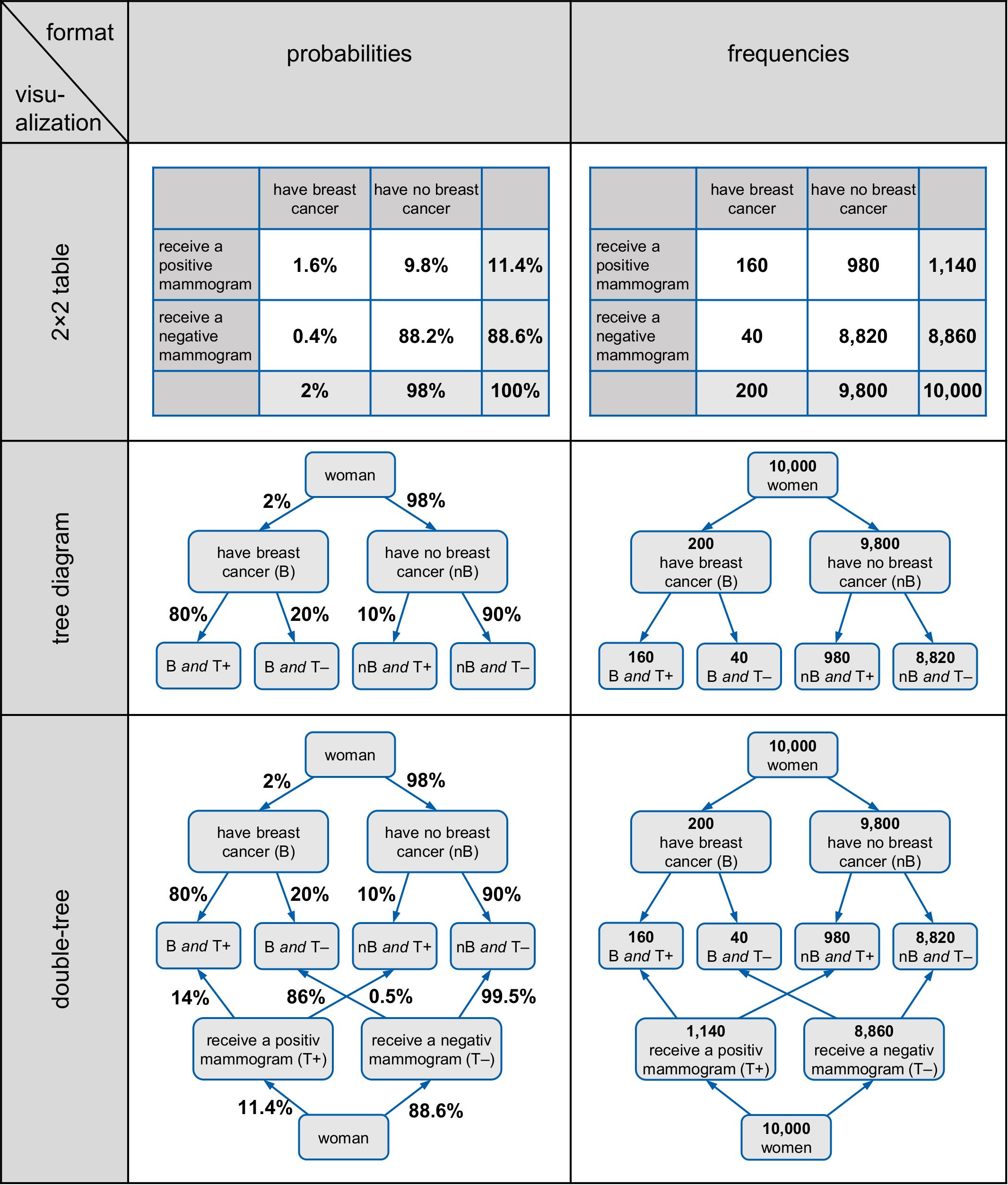
Interpretation of tree diagrams

• To find the probability of a specific path, multiply the probabilities along the branches leading to that outcome
  • Example: $P(heads \cap heads) = 0.5 \times 0.5 = 0.25$
• To find the overall probability of an outcome, sum the probabilities of all paths leading to that outcome
  • Example: $P(1 \space heads) = 0.25 + 0.25 = 0.5$
• Conditional probability can be calculated using the tree diagram
  • Identify the paths that satisfy the given condition (paths with at least one heads)
  • Sum the probabilities of these paths and divide by the probability of the given condition
    • Example: $P(at \space least \space 1 \space heads | 1st \space flip \space heads) = \frac{0.5}{0.5} = 1$
• Bayes' Theorem can be applied using tree diagrams to update the probability of an event based on new information
  • Formula: $P(A|B) = \frac{P(B|A) \times P(A)}{P(B)}$
  • Example: $P(1st \space heads | at \space least \space 1 \space heads) = \frac{0.5 \times 0.5}{0.75} = 0.333$
• Tree diagrams can illustrate the law of total probability

Fundamental Probability Concepts

• Probability axioms form the foundation of probability theory
• Events can be mutually exclusive, meaning they cannot occur simultaneously
• The law of total probability states that the probability of an event is the sum of the probabilities of all possible ways for the event to occur