9.1 Binary classification

Binary classification is a fundamental technique in image analysis, allowing computers to categorize visual data into two distinct classes. This process forms the basis for many automated decision-making tasks, from medical diagnosis to object detection in computer vision applications.

Understanding binary classification is crucial for working with Images as Data. It involves feature extraction, algorithm selection, and performance evaluation. Challenges like class imbalance and overfitting must be addressed to create effective and reliable image classification systems.

Fundamentals of binary classification

• Binary classification forms the foundation of many image analysis tasks in the field of Images as Data
• Enables computers to categorize visual information into two distinct classes, facilitating automated decision-making processes
• Serves as a crucial step in various image processing pipelines, from medical diagnosis to object detection in computer vision

Definition and purpose

Top images from around the web for Definition and purpose

• 

  Hands-on: Machine learning: classification and regression / Statistics and machine learning View original

  Is this image relevant?

• 

  Decision Trees for Machine Learning View original

  Is this image relevant?

• 

  Hands-on: Deep Learning (Part 1) - Feedforward neural networks (FNN) / Statistics and machine ... View original

  Is this image relevant?

• 

  Hands-on: Machine learning: classification and regression / Statistics and machine learning View original

  Is this image relevant?

• 

  Decision Trees for Machine Learning View original

  Is this image relevant?

1 of 3

Top images from around the web for Definition and purpose

• 

  Hands-on: Machine learning: classification and regression / Statistics and machine learning View original

  Is this image relevant?

• 

  Decision Trees for Machine Learning View original

  Is this image relevant?

• 

  Hands-on: Deep Learning (Part 1) - Feedforward neural networks (FNN) / Statistics and machine ... View original

  Is this image relevant?

• 

  Hands-on: Machine learning: classification and regression / Statistics and machine learning View original

  Is this image relevant?

• 

  Decision Trees for Machine Learning View original

  Is this image relevant?

1 of 3

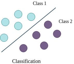
• Categorizes input data into one of two predefined classes or categories
• Utilizes machine learning algorithms to create decision boundaries between classes
• Outputs a binary prediction (0 or 1, yes or no, true or false) for each input instance
• Aims to minimize misclassification errors and maximize correct predictions

Types of binary classifiers

• Linear classifiers create a straight decision boundary to separate classes (logistic regression, linear SVM)
• Non-linear classifiers use complex decision boundaries for more intricate class separations (decision trees, neural networks)
• Probabilistic classifiers output class probabilities instead of hard decisions (Naive Bayes, logistic regression)
• Kernel-based classifiers transform input space to higher dimensions for better separation (kernel SVM)

Applications in image analysis

• Medical imaging detects presence or absence of diseases in X-rays, MRIs, or CT scans
• Facial recognition systems determine if two face images belong to the same person
• Quality control in manufacturing identifies defective products from images
• Content moderation flags inappropriate or unsafe images on social media platforms
• Satellite imagery analysis classifies land use patterns or detects changes in terrain

Feature extraction for classification

• Feature extraction transforms raw image data into meaningful representations for binary classification
• Reduces dimensionality of input data while preserving relevant information for class discrimination
• Plays a crucial role in the performance and efficiency of classification algorithms in image analysis tasks

Pixel-based features

• Raw pixel intensities serve as basic features for simple classification tasks
• Histogram of pixel values captures overall intensity distribution in an image
• Statistical moments (mean, variance, skewness) summarize pixel intensity characteristics
• Spatial relationships between pixels encoded through co-occurrence matrices
• Edge detection algorithms highlight boundaries and contours in images

Texture and edge features

• Gray Level Co-occurrence Matrix (GLCM) quantifies texture patterns in images
• Gabor filters extract texture information at different scales and orientations
• Local Binary Patterns (LBP) capture local texture patterns in a compact form
• Haralick features compute statistical measures from GLCM for texture analysis
• Edge orientation histograms summarize distribution of edge directions in an image

Color-based features

• Color histograms represent distribution of colors in different color spaces (RGB, HSV)
• Color moments capture statistical properties of color channels
• Color coherence vectors distinguish between coherent and incoherent regions of similar colors
• Dominant color descriptors identify and represent prominent colors in an image
• Color correlogram encodes spatial correlation of colors at different distances

Common binary classification algorithms

• Binary classification algorithms form the core of many image analysis tasks in the field of Images as Data
• These algorithms learn decision boundaries from training data to classify new, unseen images
• Selection of appropriate algorithm depends on the nature of the data, computational resources, and specific requirements of the image analysis task

Logistic regression

• Linear model that estimates probability of an instance belonging to a particular class
• Uses sigmoid function to map linear combinations of features to probabilities
• Decision boundary represented by a hyperplane in feature space
• Coefficients of the model indicate importance of each feature in classification
• Regularization techniques (L1, L2) prevent overfitting and improve generalization

Support vector machines

• Finds optimal hyperplane that maximizes margin between two classes
• Kernel trick allows non-linear decision boundaries through implicit feature space transformation
• Soft margin SVM tolerates some misclassifications to improve generalization
• Support vectors are critical data points that define the decision boundary
• Effective in high-dimensional spaces, common in image classification tasks

Decision trees and random forests

• Decision trees create hierarchical splits based on feature values to classify instances
• Random forests combine multiple decision trees to reduce overfitting and improve robustness
• Feature importance can be derived from the tree structure or ensemble
• Handle both numerical and categorical features without preprocessing
• Bagging and feature randomness in random forests increase diversity of trees

Performance evaluation metrics

• Performance metrics quantify the effectiveness of binary classifiers in image analysis tasks
• Different metrics capture various aspects of classifier performance, guiding model selection and optimization
• Understanding these metrics helps in interpreting results and making informed decisions in image classification projects

Accuracy vs precision

• Accuracy measures overall correctness of predictions across all classes
• Calculated as (true positives + true negatives) / total predictions
• Precision focuses on correctness of positive predictions
• Computed as true positives / (true positives + false positives)
• Precision crucial in applications where false positives are costly (medical diagnosis)

Recall and F1 score

• Recall quantifies the ability to find all positive instances
• Calculated as true positives / (true positives + false negatives)
• F1 score balances precision and recall through harmonic mean
• F1 score formula: $2 * (precision * recall) / (precision + recall)$
• Useful when dataset has imbalanced class distribution

ROC curves and AUC

• Receiver Operating Characteristic (ROC) curve plots true positive rate against false positive rate
• Visualizes trade-off between sensitivity and specificity at various classification thresholds
• Area Under the Curve (AUC) summarizes overall performance of a classifier
• AUC ranges from 0.5 (random guess) to 1.0 (perfect classification)
• Insensitive to class imbalance, useful for comparing different models

Challenges in image-based classification

• Image-based classification faces unique challenges in the field of Images as Data
• These challenges can significantly impact the performance and reliability of binary classifiers
• Addressing these issues requires careful consideration of data preparation, model selection, and evaluation strategies

Class imbalance

• Occurs when one class significantly outnumbers the other in the dataset
• Can lead to biased models that perform poorly on minority class
• Techniques to address include oversampling minority class (SMOTE)
• Undersampling majority class or using weighted loss functions
• Evaluation metrics like F1 score or AUC more appropriate for imbalanced datasets

Overfitting and underfitting

• Overfitting happens when model learns noise in training data, performs poorly on new data
• Signs include high training accuracy but low validation/test accuracy
• Underfitting occurs when model is too simple to capture underlying patterns
• Results in poor performance on both training and test data
• Regularization, cross-validation, and appropriate model complexity help mitigate these issues

Noise and outliers

• Image data often contains noise from various sources (sensor limitations, compression artifacts)
• Outliers can skew the decision boundary and reduce classifier performance
• Preprocessing techniques like median filtering or Gaussian smoothing reduce noise
• Robust loss functions (Huber loss) make models less sensitive to outliers
• Anomaly detection methods can identify and handle outliers before classification

Data preparation techniques

• Data preparation plays a crucial role in enhancing the performance of binary classifiers in image analysis
• Proper preparation techniques can significantly improve the quality and representativeness of the training data
• These techniques help address common challenges in image-based classification and improve model generalization

Image preprocessing

• Resizing normalizes image dimensions for consistent input to classifiers
• Color space conversion (RGB to grayscale) reduces dimensionality
• Histogram equalization enhances contrast and normalizes brightness
• Noise reduction techniques (Gaussian blur, median filtering) improve signal quality
• Edge enhancement (Sobel, Canny) accentuates important features for classification

Augmentation strategies

• Data augmentation artificially increases dataset size and diversity
• Geometric transformations include rotation, flipping, scaling, and translation
• Color augmentations adjust brightness, contrast, saturation, and hue
• Noise injection simulates real-world variability in image quality
• Cutout or random erasing techniques improve robustness to occlusions
• Mixup creates new training samples by linearly combining existing images

Balancing datasets

• Oversampling minority class through techniques like SMOTE (Synthetic Minority Over-sampling Technique)
• Undersampling majority class using random or informed selection methods
• Combination of over- and under-sampling (SMOTEENN, SMOTETomek)
• Class weighting in loss function to give more importance to minority class
• Ensemble methods like BalancedRandomForestClassifier for imbalanced datasets
• Stratified sampling ensures proportional representation of classes in train/test splits

Advanced binary classification methods

• Advanced binary classification methods push the boundaries of performance in image analysis tasks
• These techniques leverage complex algorithms and architectures to capture intricate patterns in image data
• Understanding and applying these methods can lead to significant improvements in classification accuracy and generalization

Ensemble learning approaches

• Combines predictions from multiple models to improve overall performance
• Bagging creates diverse models by training on different subsets of data (Random Forests)
• Boosting builds models sequentially, focusing on misclassified instances (AdaBoost, Gradient Boosting)
• Stacking uses predictions from base models as input for a meta-classifier
• Voting ensembles combine predictions through majority vote or weighted average

Deep learning for binary tasks

• Convolutional Neural Networks (CNNs) excel at extracting hierarchical features from images
• Transfer learning utilizes pre-trained CNN architectures (VGG, ResNet) for feature extraction
• Fine-tuning adapts pre-trained networks to specific binary classification tasks
• Siamese networks compare image pairs for similarity-based binary classification
• Attention mechanisms focus on relevant parts of images for improved classification

Transfer learning in classification

• Utilizes knowledge from pre-trained models on large datasets (ImageNet)
• Feature extraction freezes pre-trained layers and trains only the final classification layers
• Fine-tuning adjusts weights of pre-trained layers for task-specific optimization
• Domain adaptation techniques address differences between source and target domains
• Few-shot learning leverages transfer learning for tasks with limited labeled data

Interpreting classification results

• Interpreting classification results enhances understanding of model behavior in image analysis tasks
• These interpretation techniques provide insights into the decision-making process of binary classifiers
• Improved interpretability leads to better model refinement, debugging, and trust in the classification system

Feature importance analysis

• Identifies which features contribute most significantly to classification decisions
• Permutation importance measures impact of shuffling individual features on model performance
• SHAP (SHapley Additive exPlanations) values quantify feature contributions for individual predictions
• Gradient-based methods compute sensitivity of output with respect to input features
• Feature ablation studies remove features systematically to assess their impact

Visualization of decision boundaries

• Plots decision boundaries in feature space to understand classifier behavior
• t-SNE or UMAP reduce high-dimensional feature spaces for 2D/3D visualization
• Decision boundary plots show regions of different class predictions
• Confusion matrices visualize classification performance across different classes
• Misclassified instances plotted near decision boundaries highlight challenging cases

Explainable AI techniques

• LIME (Local Interpretable Model-agnostic Explanations) approximates local decision boundaries
• Grad-CAM generates heatmaps highlighting important regions in input images
• Concept activation vectors identify human-interpretable concepts learned by the model
• Counterfactual explanations show minimal changes needed to flip classification
• Rule extraction techniques derive interpretable rules from complex models

Practical considerations

• Practical considerations in binary classification are crucial for deploying effective image analysis systems
• These factors impact the real-world applicability and scalability of classification models
• Addressing these considerations ensures that binary classifiers can be successfully integrated into production environments

Computational efficiency

• Model complexity affects training and inference time (simpler models for real-time applications)
• GPU acceleration significantly speeds up deep learning model training and inference
• Quantization reduces model size and improves inference speed on resource-constrained devices
• Pruning removes unnecessary connections in neural networks, reducing computational requirements
• Efficient data loading and preprocessing pipelines optimize overall system performance

Scalability for large datasets

• Distributed training enables processing of large datasets across multiple machines
• Batch processing allows handling of datasets that don't fit in memory
• Online learning algorithms update models incrementally with new data
• Data sharding and parallel processing techniques improve training efficiency
• Cloud computing platforms provide scalable infrastructure for large-scale image classification tasks

Real-time classification challenges

• Low-latency requirements necessitate optimized model architectures and inference pipelines
• Edge computing brings classification closer to data sources, reducing network latency
• Model compression techniques (pruning, quantization) enable deployment on resource-constrained devices
• Streaming data processing handles continuous influx of images in real-time applications
• Caching and prediction serving frameworks optimize model deployment for high-throughput scenarios

Ethical implications

• Ethical considerations in binary classification are paramount in the field of Images as Data
• These implications impact the fairness, privacy, and societal effects of image analysis systems
• Addressing ethical concerns ensures responsible development and deployment of binary classifiers

Bias in training data

• Dataset bias can lead to unfair or discriminatory classification results
• Demographic bias results in poor performance for underrepresented groups
• Historical bias perpetuates existing societal prejudices through automated decisions
• Sampling bias occurs when training data doesn't represent the true population distribution
• Mitigation strategies include diverse data collection and bias-aware model development

Privacy concerns

• Image data often contains sensitive personal information (facial features, location data)
• Anonymization techniques (blurring, pixelation) protect individual privacy in datasets
• Federated learning enables model training without centralizing sensitive data
• Differential privacy adds controlled noise to protect individual data points
• Secure multi-party computation allows collaborative learning while preserving data privacy

Responsible use of classifiers

• Transparency in model decisions and limitations crucial for ethical deployment
• Regular audits assess fairness and potential biases in classification systems
• Human-in-the-loop approaches incorporate human judgment in critical decisions
• Clear documentation of model capabilities and intended use cases prevents misuse
• Ongoing monitoring and updating of models address emerging ethical concerns