ARMA models blend past values and errors to predict future outcomes in time series data. They combine autoregressive (AR) and (MA) components, capturing both historical trends and recent fluctuations.

Understanding ARMA models is crucial for forecasting stationary time series. By grasping their structure, characteristics, and forecasting process, you'll be better equipped to analyze and predict patterns in various fields, from finance to environmental studies.

ARMA model foundations

Composition and structure of ARMA models

Top images from around the web for Composition and structure of ARMA models
  • ARMA models combine autoregressive (AR) and moving average (MA) components capturing both the dependence on past values and the influence of past forecast errors
  • The AR component represents the relationship between an observation and a specified number of lagged observations (pp)
  • The MA component represents the error of the model as a combination of previous error terms with a specified number of lags (qq)
  • ARMA models are denoted as ARMA(pp,qq) where pp is the order of the autoregressive term and qq is the order of the moving average term
  • The general form of an ARMA(pp,qq) model is:
    • Xt=c+โˆ‘i=1pฯ•iXtโˆ’i+โˆ‘i=1qฮธiฮตtโˆ’i+ฮตtX_t = c + \sum_{i=1}^{p} \phi_i X_{t-i} + \sum_{i=1}^{q} \theta_i \varepsilon_{t-i} + \varepsilon_t
    • XtX_t is the time series value at time tt
    • cc is a constant term
    • ฯ•i\phi_i and ฮธi\theta_i are model parameters
    • ฮตt\varepsilon_t is (random error) at time tt

Stationarity assumption in ARMA models

  • ARMA models assume the time series is stationary meaning its statistical properties (mean, variance, autocovariance) do not change over time
  • is crucial for the model to capture the underlying patterns and relationships in the data accurately
  • Non-stationary time series can lead to spurious relationships and unreliable forecasts
  • Stationarity can be assessed using visual inspection (time series plot), statistical tests (Augmented Dickey-Fuller, KPSS), or examining ACF and PACF plots
  • If the time series is non-stationary, transformations such as or detrending can be applied to achieve stationarity before fitting an

ARMA model characteristics

Autoregressive (AR) component

  • The AR component captures the linear dependence between an observation and its past values
  • The order pp determines the number of lagged observations included in the model
  • Higher values of pp indicate a stronger dependence on past observations
  • The AR component is represented by the term โˆ‘i=1pฯ•iXtโˆ’i\sum_{i=1}^{p} \phi_i X_{t-i} in the ARMA equation
  • The parameters ฯ•i\phi_i determine the weights assigned to the lagged observations

Moving average (MA) component

  • The MA component represents the error of the model as a linear combination of past forecast errors
  • The order qq determines the number of lagged errors included in the model
  • Higher values of qq indicate a stronger influence of past forecast errors
  • The MA component is represented by the term โˆ‘i=1qฮธiฮตtโˆ’i\sum_{i=1}^{q} \theta_i \varepsilon_{t-i} in the ARMA equation
  • The parameters ฮธi\theta_i determine the weights assigned to the lagged errors

Additional components and parameters

  • The constant term cc in the ARMA model represents the mean of the time series if it is non-zero
  • The white noise term ฮตt\varepsilon_t represents the random error or innovation at time tt assumed to be independently and identically distributed with a mean of zero and constant variance
  • The parameters ฯ•i\phi_i and ฮธi\theta_i are estimated using methods such as maximum likelihood estimation or least squares to minimize the difference between the observed and predicted values

ARMA model forecasting

Model development process
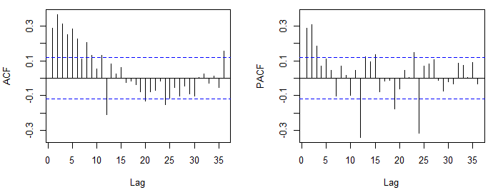
  • Determine the appropriate orders (pp and qq) using tools such as the function (ACF) and partial autocorrelation function (PACF)
    • ACF measures the correlation between observations at different lags
    • PACF measures the correlation between observations at different lags while controlling for the effects of intermediate lags
  • Estimate the model parameters (ฯ•i\phi_i and ฮธi\theta_i) using suitable methods like maximum likelihood estimation or least squares ensuring the estimated parameters are statistically significant
  • Assess the model's goodness of fit using diagnostic tests such as the Ljung-Box test for residual autocorrelation and the Akaike Information Criterion (AIC) or Bayesian Information Criterion () for

Interpretation and forecasting

  • Interpret the estimated parameters to understand the influence of past observations and errors on the current value of the time series
    • Positive ฯ•i\phi_i values indicate a positive relationship between the current observation and the ii-th lagged observation
    • Negative ฮธi\theta_i values indicate a negative relationship between the current observation and the ii-th lagged error
  • Use the developed ARMA model to generate forecasts for future time periods
  • Assess the accuracy of these forecasts using appropriate evaluation metrics such as mean squared error (MSE) or mean absolute percentage error (MAPE)
    • MSE measures the average squared difference between the observed and predicted values
    • MAPE measures the average absolute percentage difference between the observed and predicted values

Stationarity vs Invertibility in ARMA models

Stationarity requirement

  • ARMA models require the time series to be stationary meaning its statistical properties (mean, variance, autocovariance) do not change over time
  • Stationarity ensures the model captures the underlying patterns and relationships in the data accurately
  • Non-stationary time series can lead to spurious relationships and unreliable forecasts
  • If the time series is non-stationary, transformations such as differencing or detrending can be applied to achieve stationarity before fitting an ARMA model
    • Differencing involves computing the differences between consecutive observations to remove trends
    • Detrending involves removing deterministic trends (linear, quadratic) from the time series

Invertibility requirement

  • Invertibility is a requirement for the MA component of the ARMA model ensuring the model can be expressed as an infinite sum of past observations
  • The invertibility condition is satisfied when the absolute values of the roots of the MA characteristic equation lie outside the unit circle
    • MA characteristic equation: 1โˆ’โˆ‘i=1qฮธizi=01 - \sum_{i=1}^{q} \theta_i z^i = 0
    • The roots of this equation should have absolute values greater than 1
  • Non-invertible ARMA models can lead to identifiability issues and unreliable parameter estimates making it crucial to ensure invertibility before interpreting and using the model for forecasting
  • Invertibility can be checked by examining the roots of the MA characteristic equation or by assessing the model's residuals for independence and normality

Key Terms to Review (17)

ARMA Model: An ARMA model, or Autoregressive Moving Average model, is a statistical method used to analyze and forecast time series data by combining two components: autoregression (AR) and moving averages (MA). This model is essential for capturing the relationship between an observation and a number of lagged observations as well as the relationship between an observation and a residual error from a moving average model, making it valuable for understanding temporal dependencies in data.
Autocorrelation: Autocorrelation refers to the correlation of a time series with its own past values. It measures how current values in a series are related to its previous values, helping to identify patterns or trends over time. Understanding autocorrelation is essential for analyzing data, as it affects the selection of forecasting models and their accuracy.
Autoregressive model: An autoregressive model is a statistical representation that uses the dependency between an observation and a number of lagged observations (previous time periods) to predict future values. This approach emphasizes how past values influence current data points, making it essential for analyzing time series data. It is a foundational concept in time series analysis and plays a crucial role in autoregressive moving average models, where both autoregressive and moving average components are combined for more accurate forecasting.
BIC: BIC, or Bayesian Information Criterion, is a statistical tool used for model selection that evaluates how well a model explains the data while penalizing for the number of parameters used. It helps in determining the best-fitting model among a set of candidates by balancing goodness-of-fit and complexity. Lower BIC values indicate a more favorable model, making it a valuable criterion in the context of autoregressive models, moving averages, and integrated models.
Differencing: Differencing is a technique used in time series analysis to transform non-stationary data into stationary data by subtracting the previous observation from the current observation. This method helps in stabilizing the mean of the time series by removing trends or seasonal patterns, making it easier to analyze and forecast future values. It plays a crucial role in enhancing the performance of various forecasting models by ensuring that the assumptions of stationarity are met.
G. m. jenkins: G. M. Jenkins is a notable figure in the field of time series analysis, particularly known for his contributions to the development of statistical methods for modeling time-dependent data. His work laid foundational principles that have influenced various forecasting techniques, especially in the context of Autoregressive Moving Average (ARMA) models, where he provided insights into the model's behavior and applicability to real-world scenarios.
George E.P. Box: George E.P. Box was a renowned statistician known for his significant contributions to time series analysis and forecasting methods. His work laid the foundation for many statistical models and techniques used in data analysis today, connecting various concepts such as components of time series, moving averages, and state space models in forecasting.
Homoscedasticity: Homoscedasticity refers to a key assumption in regression analysis where the variance of the residuals, or errors, is constant across all levels of an independent variable. This concept is crucial because if homoscedasticity holds true, it indicates that the modelโ€™s predictions are reliable and the relationship between the dependent and independent variables remains consistent. When this assumption is violated, it can lead to inefficient estimates and affect hypothesis tests, causing misleading conclusions.
Linearity: Linearity refers to the property of a relationship where changes in one variable lead to proportional changes in another variable, often depicted as a straight line in a graph. This concept is crucial in understanding how variables interact, making it easier to model and predict outcomes in various analytical frameworks. In statistical modeling, maintaining linearity ensures that predictions are reliable and interpretations are straightforward.
Model selection: Model selection is the process of choosing the best statistical model from a set of candidate models to represent a given data set and make accurate forecasts. This involves evaluating the performance of different models based on criteria such as predictive accuracy, complexity, and interpretability. The goal is to find a model that effectively captures the underlying patterns in the data while avoiding overfitting.
Moving average: A moving average is a statistical calculation used to analyze data points by creating averages of different subsets of the full dataset over time. This method smooths out short-term fluctuations and highlights longer-term trends, making it a crucial tool in understanding time series data, forecasting future values, and assessing the accuracy of predictions.
Parameter estimation: Parameter estimation is a statistical technique used to determine the values of parameters within a model that best fit a set of observed data. This process involves estimating coefficients that define the relationships between variables, allowing for accurate predictions and analyses. It is crucial in various modeling approaches, as it directly influences the quality and reliability of forecasts generated by those models.
Python: Python is a high-level programming language known for its simplicity and versatility, making it a popular choice for data analysis, machine learning, and statistical modeling. Its rich ecosystem of libraries allows users to implement complex forecasting models easily and efficiently, which is crucial in areas such as multiple linear regression, time series analysis, and hierarchical forecasting.
R: In the context of forecasting and regression analysis, 'r' typically represents the correlation coefficient, which quantifies the degree to which two variables are linearly related. This statistic is crucial for understanding relationships in time series data, assessing model fit, and evaluating the strength of predictors in regression models. Its significance extends across various forecasting methods, helping to gauge accuracy and inform decision-making.
Seasonal Decomposition: Seasonal decomposition is a statistical method used to break down a time series into its individual components, specifically the trend, seasonal effects, and residuals. This technique helps in understanding and analyzing the underlying patterns in data, making it easier to forecast future values by separating the consistent seasonal patterns from other fluctuations. By isolating these components, it's possible to apply various modeling approaches to accurately capture the dynamics of the data.
Stationarity: Stationarity refers to a property of a time series where its statistical properties, like mean and variance, remain constant over time. This concept is crucial because many forecasting models assume that the underlying data generating process does not change, allowing for reliable predictions and inferences.
White Noise: White noise refers to a random signal with a constant power spectral density across a wide range of frequencies, meaning it contains equal intensity at different frequencies, making it useful in various time series analyses. This concept is crucial in assessing the randomness of a time series and is a foundational element in understanding the properties of stationary and non-stationary processes, as well as in the formulation of various forecasting models.
ยฉ 2024 Fiveable Inc. All rights reserved.
APยฎ and SATยฎ are trademarks registered by the College Board, which is not affiliated with, and does not endorse this website.