2.4 Marginal and conditional probability distributions

Marginal and conditional probability distributions are essential tools for understanding relationships between random variables. They help break down complex joint distributions, allowing us to focus on specific variables or conditions. These concepts are crucial for analyzing data and making informed decisions in various fields.

By deriving marginal distributions and calculating conditional probabilities, we can gain valuable insights into the behavior of individual variables. This knowledge is fundamental for probability theory and forms the basis for more advanced statistical techniques used in data analysis and machine learning.

Marginal and Conditional Distributions

Probability Distributions and Their Relationships

Top images from around the web for Probability Distributions and Their Relationships

• 

  probability or statistics - Obtaining joint distributions and conditional distributions using ... View original

  Is this image relevant?

• 

  Conditional probability distribution - Wikipedia View original

  Is this image relevant?

• 

  Assignment 3 - 2011 - Solution - Statistics for Engineering View original

  Is this image relevant?

• 

  probability or statistics - Obtaining joint distributions and conditional distributions using ... View original

  Is this image relevant?

• 

  Conditional probability distribution - Wikipedia View original

  Is this image relevant?

1 of 3

Top images from around the web for Probability Distributions and Their Relationships

• 

  probability or statistics - Obtaining joint distributions and conditional distributions using ... View original

  Is this image relevant?

• 

  Conditional probability distribution - Wikipedia View original

  Is this image relevant?

• 

  Assignment 3 - 2011 - Solution - Statistics for Engineering View original

  Is this image relevant?

• 

  probability or statistics - Obtaining joint distributions and conditional distributions using ... View original

  Is this image relevant?

• 

  Conditional probability distribution - Wikipedia View original

  Is this image relevant?

1 of 3

• A marginal probability distribution is the probability distribution of a single random variable, obtained by summing or integrating the joint probability distribution over all possible values of the other random variables
• A conditional probability distribution is the probability distribution of a random variable given the occurrence of a specific event or the value of another random variable
• Marginal and conditional probability distributions are derived from joint probability distributions, which describe the probabilities of all possible combinations of values for two or more random variables
• Example: In a joint distribution of two dice rolls, the marginal distribution of the first die would be the probabilities of each outcome (1-6) regardless of the outcome of the second die

Applications and Importance

• Marginal and conditional distributions allow for a more focused analysis of individual variables within a larger joint distribution
• They provide insights into the behavior and relationships between random variables
• Marginal distributions are useful for understanding the overall probability distribution of a single variable, while conditional distributions help in analyzing the probability of one variable given specific values of another
• Example: In a medical study, the marginal distribution of a disease prevalence can be derived from the joint distribution of disease status and risk factors, while the conditional distribution of disease status given a specific risk factor can help identify high-risk groups

Deriving Marginal Distributions

Discrete Random Variables

• To obtain the marginal probability distribution of a random variable X from a joint probability distribution $P(X, Y)$, sum the joint probabilities over all possible values of Y for each value of X
• The marginal probability distribution for discrete random variables is calculated using the formula: $P(X = x) = \sum P(X = x, Y = y)$ for all y
• Example: In a joint distribution table of two binary variables X and Y, the marginal distribution of X is obtained by summing the probabilities in each row corresponding to X=0 and X=1

Continuous Random Variables

• For continuous random variables, the marginal probability distribution is calculated using the formula: $f(x) = \int f(x, y) dy$, where $f(x, y)$ is the joint probability density function
• To derive the marginal probability density function, integrate the joint probability density function over the range of the other variable
• The resulting marginal probability density function represents the probability distribution of the variable of interest, independent of the other variable
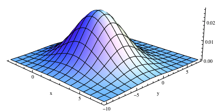
• Example: In a bivariate normal distribution with joint probability density function $f(x, y)$, the marginal distribution of X is obtained by integrating $f(x, y)$ with respect to y over its entire range

Properties of Marginal Distributions

• The marginal probability distributions of all random variables in a joint distribution must sum to 1, as they represent the total probability of each individual variable
• Marginal distributions provide a summary of the probability distribution of a single variable, without considering the effects of other variables
• Marginal distributions can be used to calculate summary statistics (mean, variance) for individual variables
• Example: The sum of the marginal probabilities of a discrete random variable X, $\sum P(X = x)$ for all x, equals 1

Calculating Conditional Probabilities

Definition and Formula

• Conditional probability is the probability of an event A occurring given that another event B has already occurred, denoted as $[P(A|B)](https://www.fiveableKeyTerm:p(a|b))$
• For discrete random variables, the conditional probability is calculated using the formula: $P(X = x|Y = y) = \frac{P(X = x, Y = y)}{P(Y = y)}$, where $P(X = x, Y = y)$ is the joint probability and $P(Y = y)$ is the marginal probability of Y
• For continuous random variables, the conditional probability density function is calculated using the formula: $f(x|y) = \frac{f(x, y)}{f(y)}$, where $f(x, y)$ is the joint probability density function and $f(y)$ is the marginal probability density function of Y

Interpreting Conditional Probabilities

• Conditional probabilities provide information about the relationship between random variables and how the probability of one variable changes based on the value of another
• They allow for updating probabilities based on new information or evidence
• Conditional probabilities are useful in various fields, such as medical diagnosis (probability of a disease given symptoms), machine learning (probability of a class given features), and decision-making (probability of an outcome given a choice)
• Example: In a medical context, the conditional probability $P(\text{Disease} | \text{Positive Test})$ represents the probability that a person has a disease given that they tested positive

Independence and Conditional Probability

• Two events A and B are considered independent if the occurrence of one does not affect the probability of the other, i.e., $P(A|B) = P(A)$ and $P(B|A) = P(B)$
• For independent events, the joint probability is equal to the product of the individual probabilities: $P(A, B) = P(A) \times P(B)$
• If events are not independent, conditional probabilities are used to describe their relationship and update probabilities based on new information
• Example: In a deck of cards, drawing a king on the first draw and drawing a queen on the second draw (without replacement) are not independent events, as the probability of drawing a queen on the second draw is affected by the outcome of the first draw

Bayes' Theorem for Probability Updates

Bayes' Theorem Formula

• Bayes' theorem is a fundamental rule in probability theory that describes how to update the probability of an event based on new information or evidence
• The theorem states that the posterior probability of an event A given evidence B is proportional to the product of the prior probability of A and the likelihood of B given A: $P(A|B) = \frac{P(B|A) \times P(A)}{P(B)}$
• In Bayes' theorem, $P(A)$ is the prior probability of event A, $P(B|A)$ is the likelihood of evidence B given event A, and $P(B)$ is the marginal probability of evidence B

Components of Bayes' Theorem

• Prior probability: The initial probability of an event A before considering any new evidence, denoted as $P(A)$
• Likelihood: The probability of observing evidence B given that event A has occurred, denoted as $P(B|A)$
• Marginal probability: The overall probability of observing evidence B, calculated by summing or integrating the joint probabilities of B and all possible events: $P(B) = \sum P(B|A_i) \times P(A_i)$ for discrete events, or $P(B) = \int P(B|A) \times P(A) dA$ for continuous events
• Posterior probability: The updated probability of event A after considering the new evidence B, denoted as $P(A|B)$

Applying Bayes' Theorem

• To apply Bayes' theorem, first identify the prior probability, likelihood, and marginal probability based on the given information
• Calculate the posterior probability using the formula: $P(A|B) = \frac{P(B|A) \times P(A)}{P(B)}$
• The posterior probability represents the updated belief or probability of event A after considering the new evidence B
• Bayes' theorem is widely used in various fields, including statistics, machine learning, and decision-making, to update beliefs or probabilities based on new data or observations
• Example: In a medical context, Bayes' theorem can be used to update the probability of a disease given a positive test result, by considering the prior probability of the disease, the likelihood of a positive test given the disease, and the marginal probability of a positive test result