Graph Representation Methods
Graphs model relationships between entities, and how you store a graph in memory directly affects the speed and memory cost of every operation you run on it. This section covers the four main representation methods, their trade-offs, and how to pick the right one for a given problem.
Adjacency matrices for graph representation
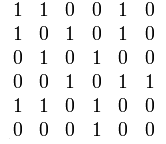
An adjacency matrix stores a graph as a 2D array of size , where is the number of vertices. Each entry is 1 if there's an edge from vertex to vertex , and 0 otherwise.
For weighted graphs, you store the edge weight instead of 1, and use a sentinel value (like 0 or ) for missing edges.
A few properties to keep in mind:
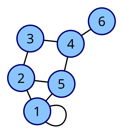
- Undirected graphs produce symmetric matrices, since an edge between and means . Think of a friendship graph: if Alice is friends with Bob, Bob is friends with Alice.
- Directed graphs can have asymmetric matrices. A hyperlink from page A to page B doesn't mean page B links back to A.
- Space complexity is always , no matter how many edges exist. That's fine for dense graphs (like a fully connected social network), but wasteful for sparse ones (like a road network where most cities connect to only a handful of neighbors).
The big advantage of adjacency matrices is constant-time edge lookup: checking whether an edge exists between any two vertices is just an array access at , which takes .
Adjacency lists vs matrices
An adjacency list uses an array of size , where each slot holds a list (linked list, dynamic array, etc.) of that vertex's neighbors.
How edges are stored depends on the graph type:
- In an undirected graph, each edge appears twice. An edge between vertices 2 and 5 shows up in vertex 2's list and vertex 5's list.
- In a directed graph, each edge appears once, in the source vertex's list. An edge from vertex 3 to vertex 7 only appears in vertex 3's list.
The space complexity is , which is much better than when the graph is sparse.
Time complexity comparison for common operations:
| Operation | Adjacency List | Adjacency Matrix |
|---|---|---|
| Add an edge | ||
| Remove an edge | ||
| Check if edge exists | ||
| Iterate over neighbors of |
A correction from the original: removing or checking an edge in an adjacency list costs (the degree of the vertex, i.e., the length of that vertex's neighbor list), not . You only scan one vertex's list, not every edge in the graph.
That last row matters a lot. Iterating over a vertex's neighbors is one of the most common operations in graph algorithms (BFS, DFS, Dijkstra's). With an adjacency list, you touch only the actual neighbors. With a matrix, you scan the entire row of entries, most of which may be zeros in a sparse graph.
Edge lists and incidence matrices
Edge lists are the simplest representation. You store an array of edge pairs, like [(1, 2), (2, 3), (1, 4)]. For weighted graphs, each entry becomes a triple: (u, v, weight).
- Space complexity:
- Great for algorithms that process edges one at a time, like Kruskal's minimum spanning tree algorithm, which sorts all edges by weight.
- Poor for adjacency queries. Checking whether a specific edge exists or finding all neighbors of a vertex requires scanning the entire list, taking time.
Incidence matrices use a 2D array of size . Each column represents an edge, and each row represents a vertex. Entry if vertex is an endpoint of edge .
- Space complexity: , which can be very large.
- Useful in specialized contexts like network flow problems or algebraic graph theory, where you need to reason about the relationship between vertices and specific edges.
- Checking if two specific vertices share an edge is slow, since you'd need to scan columns looking for a column where both vertices have a 1.
In practice, edge lists and incidence matrices are less commonly used than adjacency lists and matrices, but they show up in specific algorithmic contexts.
Selecting graph representation methods
Picking the right representation comes down to three factors: graph density, which operations you'll perform most, and memory budget.
Graph density:
- Dense graphs (edge count close to ) pair well with adjacency matrices. A complete graph on 1,000 vertices has about 500,000 edges, and the matrix uses entries, which isn't much overhead.
- Sparse graphs (edge count close to ) pair well with adjacency lists or edge lists. A tree with 1,000 vertices has only 999 edges, so an adjacency list uses far less memory than a million-entry matrix.
Operation frequency:
- If you frequently check whether a specific edge exists, adjacency matrices give you lookups.
- If you frequently iterate over neighbors (as in BFS/DFS), adjacency lists are faster because you skip non-neighbors entirely.
- If you need to process all edges in bulk (sorting them, filtering them), an edge list keeps things simple.
Space constraints:
- Adjacency lists at and edge lists at are the most memory-efficient options for sparse graphs.
- Adjacency matrices always cost regardless of edge count.
Problem-specific needs:
- Algorithms like Kruskal's that sort or iterate over all edges work naturally with edge lists.
- Dynamic graphs with frequent insertions and deletions favor adjacency lists.
- Problems requiring fast pairwise adjacency checks (like verifying whether a graph is complete) favor adjacency matrices.