🧮Combinatorics Unit 5 Review
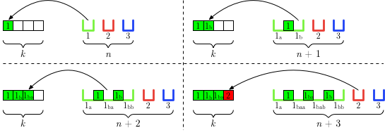
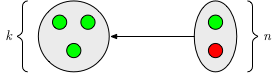
5.4 Generalizations and variations of the principle
5.4 Generalizations and variations of the principle
Unit & Topic Study Guides
Combinatorics: Sum and Product Rules Intro
Permutations and Combinations
Binomial Coefficients and Theorem
The Pigeonhole Principle and Ramsey Theory
The Principle of Inclusion–Exclusion
Generating Functions
Recurrence Relations
Partitions and Stirling Numbers
Posets and Lattices
Graph Theory Fundamentals
Paths, Cycles, and Connectivity in Graphs
Graph Coloring and Ramsey Numbers
Design Theory and Combinatorial Designs
Combinatorial Optimization & Network Flows
Applications in Probability and Statistics
Inclusion-Exclusion Principle
Multiset Inclusion-Exclusion
Standard PIE counts elements across distinct sets, but many counting problems involve elements that can appear more than once. Multiset PIE adapts the framework to handle these repeated elements by weighting intersections according to element multiplicities.
The core idea: when you're counting arrangements or selections from a multiset (a set where repetition is allowed), you still alternate between adding and subtracting overcounted terms. But each term now accounts for how many times elements appear, not just whether they appear.
- Solves problems like permutations with repetition and distributing identical objects into distinct bins
- Uses complementary counting alongside multiset PIE to simplify problems with upper-bound constraints
- Pairs naturally with the "stars and bars" method when restrictions are placed on individual bins
Example: Suppose you want to distribute 10 identical balls into 5 distinct boxes, where each box must contain between 1 and 4 balls. You'd start with the unrestricted count (stars and bars), then use PIE to subtract the cases where one or more boxes exceed 4, adding back the cases where two or more boxes exceed 4, and so on.
Applications in Function Counting
One of the most important uses of PIE is counting surjective (onto) functions, where every element in the codomain is mapped to by at least one element in the domain.
The strategy is to count by complement. Let be the set of functions from an -element domain to an -element codomain that miss codomain element . Then PIE gives the number of surjections as:
Each term counts the functions that miss at least a specific set of codomain elements. The alternating sum corrects for overcounting.
- The formula connects directly to Stirling numbers of the second kind: the number of surjections from an -set to an -set equals
- Restricted codomain problems add further constraints on which codomain elements must or must not appear in the range
- Applications include task assignment, cryptographic mappings, and data compression schemes
Example: To assign 20 tasks to 5 workers so that every worker gets at least one task, you'd compute .
Applications of Inclusion-Exclusion
Complex Set Relationships
Generalized PIE extends the standard formula to handle situations where set memberships are dependent or where you need to consider intersections of a specific size.
- k-wise intersections: Sometimes you only need to account for intersections involving or more sets simultaneously. Truncating the PIE sum at a certain depth gives useful bounds (more on this in the Bonferroni section below).
- Weighted sets: When elements contribute different values rather than just being "in" or "out," PIE can be adapted so that each intersection term carries a weight reflecting those values.
- Generating functions: For problems with complex constraints or infinitely many cases, you can encode the inclusion-exclusion structure inside a generating function. The coefficients of the resulting series give your counts directly.
- Conditional dependence: When set membership in one set affects membership in another, you modify the PIE formula to incorporate conditional probabilities at each intersection term.
Example: Computing the probability of at least one success in a series of dependent trials requires adjusting each intersection term to reflect the dependence structure, rather than assuming independence.
Graph Theory Applications
PIE is a key tool in graph coloring and related structural problems.
The chromatic polynomial gives the number of proper colorings of a graph using colors (where no two adjacent vertices share a color). PIE constructs this polynomial by systematically subtracting colorings that violate edge constraints:
- Start with total colorings of vertices (ignoring edges).
- For each edge, subtract colorings where both endpoints share a color.
- Add back colorings where two or more edges simultaneously have matching endpoints.
- Continue alternating until all edges are accounted for.
The result is a polynomial in that works for any number of colors.
- Also applies to counting independent sets (sets of vertices with no edges between them) and dominating sets
- Scheduling problems often reduce to graph coloring: vertices are tasks, edges represent conflicts, and colors represent time slots or resources
Example: Assigning frequencies to radio stations so that nearby stations don't interfere is a graph coloring problem. PIE helps count (or bound) the number of valid frequency assignments.
Variations of Inclusion-Exclusion
Sieve Methods
The connection between PIE and sieve methods in number theory is deep and practical.
The Sieve of Eratosthenes is essentially PIE in action. To count primes up to :
- List all integers from 2 to .
- Let be the set of multiples of prime (excluding itself) for each prime .
- Apply PIE to count integers in (the composites).
- Subtract from to get the prime count.
This PIE perspective generalizes to other sieves:
- Sieve of Sundaram: Eliminates certain integers of a specific form to produce odd primes
- Legendre's formula: Directly applies PIE with prime factor sets to count primes in a range
- More advanced analytic sieves (Brun's sieve, Selberg's sieve) refine the PIE approach by using optimized weights on the intersection terms to get tighter bounds
Example: Finding all primes less than 100 requires sieving out multiples of primes up to , so you only need to eliminate multiples of 2, 3, 5, and 7.
Bonferroni Inequalities
When a full PIE calculation involves too many terms to be practical, Bonferroni inequalities let you truncate the alternating sum and still get useful bounds.
The key property of PIE's alternating sum is that truncating after an odd number of terms gives an upper bound, while truncating after an even number of terms gives a lower bound on .
- The first-order Bonferroni bound is just the union bound:
- The second-order bound subtracts pairwise intersections, giving a lower bound
- Each additional level of terms tightens the bound, alternating between over- and underestimates
- These bounds are especially valuable in statistics for multiple hypothesis testing, where you need to control the probability of at least one false positive across many tests (family-wise error rate)
- They also extend to continuous settings in measure theory and probability density estimation
Example: In quality control, if you have 1000 items each with a small defect probability, computing the exact probability that at least one is defective requires enormous PIE sums. The first Bonferroni bound gives a quick upper estimate, and the second bound gives a lower estimate, often sufficient for practical decisions.