5.2 The Definite Integral

The Definite Integral

Components of a Definite Integral

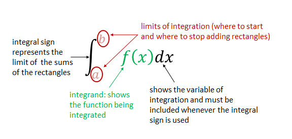
A definite integral calculates the accumulated value of a function over a specific interval. The full notation is $\int_a^b f(x)\, dx$, and each piece has a role:

• Integrand $f(x)$: the function being integrated
• Lower limit $a$: where the interval starts
• Upper limit $b$: where the interval ends
• Differential $dx$: tells you the variable of integration

The definite integral is formally defined as the limit of a Riemann sum. You partition the interval $[a, b]$ into $n$ subintervals, each of width $\Delta x = \frac{b - a}{n}$, then pick a sample point $x_i^*$ in each subinterval and form the sum:

$\sum_{i=1}^{n} f(x_i^*)\, \Delta x$

As $n \to \infty$, this sum converges to the exact value of the definite integral. Each term $f(x_i^*)\, \Delta x$ represents the area of a thin rectangle, so the Riemann sum is really just an approximation that gets better as the rectangles get thinner.

Integrability of Functions

A function $f(x)$ is integrable on $[a, b]$ if the limit of its Riemann sums exists and converges to a single value, no matter how you choose the sample points $x_i^*$. Both left and right Riemann sums (and any other sampling method) must approach the same number.

If a function is not integrable, different choices of sample points can give different limiting values, which means the definite integral isn't well-defined.

The most important guarantee: if $f(x)$ is continuous on $[a, b]$, then it's integrable on that interval. Functions with a finite number of jump discontinuities are also integrable, but continuous functions are the case you'll encounter most often in this course.

Definite Integrals as Net Area

The definite integral $\int_a^b f(x)\, dx$ gives the net area between the graph of $f(x)$ and the $x$-axis over $[a, b]$.

• When $f(x) \geq 0$ on the entire interval, the integral equals the total area under the curve.
• When $f(x)$ dips below the $x$-axis, those regions contribute negative area. The integral then equals (area above the axis) minus (area below the axis).

This distinction between net area and total area trips people up. If you want the total area (ignoring sign), you'd integrate $|f(x)|$ instead. But the definite integral itself always gives net area.

This geometric interpretation also means you can evaluate some definite integrals without any algebra. For example, $\int_{-3}^{3} \sqrt{9 - x^2}\, dx$ represents the area of a semicircle with radius 3, which is $\frac{9\pi}{2}$.

Fundamental Concepts

• Accumulation: The definite integral represents the total accumulation of a quantity over an interval. Think of it as adding up infinitely many infinitesimally small contributions.
• Limit process: The precise definition relies on taking the limit of Riemann sums as $n \to \infty$. This is what turns an approximation into an exact answer.
• The framework is named after Bernhard Riemann, who formalized the idea of partitioning intervals and summing function values to define integration rigorously.

Evaluating and Interpreting Definite Integrals

Evaluation Methods

The main tool for evaluating definite integrals is the Fundamental Theorem of Calculus (Part 1):

$\int_a^b f(x)\, dx = F(b) - F(a)$

where $F(x)$ is any antiderivative of $f(x)$. This connects differentiation and integration: instead of computing a limit of Riemann sums, you find an antiderivative and plug in the bounds.

Steps to evaluate using the FTC:

1. Find an antiderivative $F(x)$ of the integrand $f(x)$.
2. Evaluate $F(b)$ (antiderivative at the upper limit).
3. Evaluate $F(a)$ (antiderivative at the lower limit).
4. Subtract: $F(b) - F(a)$.

For example, to evaluate $\int_1^4 x^2\, dx$: the antiderivative is $F(x) = \frac{x^3}{3}$, so the result is $\frac{64}{3} - \frac{1}{3} = \frac{63}{3} = 21$.

Key properties that simplify evaluation:

• Linearity: $\int_a^b [c\, f(x) + d\, g(x)]\, dx = c\int_a^b f(x)\, dx + d\int_a^b g(x)\, dx$. You can pull out constants and split sums.
• Additivity: $\int_a^b f(x)\, dx + \int_b^c f(x)\, dx = \int_a^c f(x)\, dx$. You can break an interval into pieces or combine adjacent integrals.
• Reversing limits: $\int_a^b f(x)\, dx = -\int_b^a f(x)\, dx$. Swapping the limits flips the sign.
• Zero-width interval: $\int_a^a f(x)\, dx = 0$. No interval means no accumulation.

Average Value Through Definite Integrals

The average value of $f(x)$ on $[a, b]$ is:

$f_{\text{avg}} = \frac{1}{b - a} \int_a^b f(x)\, dx$

The logic here is straightforward: the integral gives the total accumulated value, and dividing by the interval width $b - a$ gives the average height of the function.

For example, if the temperature over a 12-hour period is modeled by $T(t)$, then $\frac{1}{12}\int_0^{12} T(t)\, dt$ gives the average temperature during that period.

Physical interpretations come up frequently:

• Average velocity over a time interval (physics)
• Average cost per unit over a production range (economics)
• Average concentration of a substance over time (chemistry)

The Mean Value Theorem for Integrals guarantees that if $f$ is continuous on $[a, b]$, there exists at least one point $c$ in $[a, b]$ where $f(c)$ equals the average value. In other words, the function actually hits its average somewhere on the interval.