models blend , , and components to forecast time series data. The method offers a step-by-step approach to identify, estimate, and diagnose these models, aiming for simplicity and accuracy in describing data.

Model identification involves examining and plots to determine model order, while avoiding overfitting. Parameter estimation uses maximum likelihood methods to find optimal values. Information criteria like and help select the best model, balancing fit and complexity.

ARIMA Model Identification

Understanding ARIMA Models and Box-Jenkins Methodology

Top images from around the web for Understanding ARIMA Models and Box-Jenkins Methodology
  • ARIMA models combine autoregressive (AR), differencing (I), and moving average (MA) components to forecast time series data
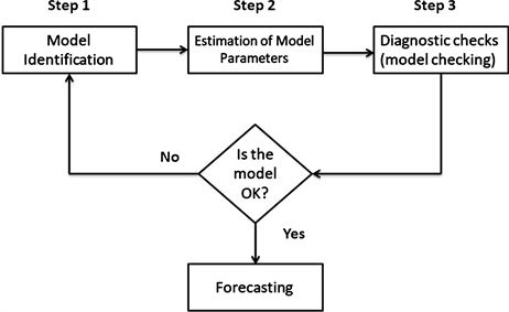
  • Box-Jenkins methodology provides a systematic approach for identifying, estimating, and diagnosing ARIMA models
  • Process involves iterative steps of model identification, parameter estimation, and diagnostic checking
  • Aims to find the most parsimonious model that adequately describes the data (balances simplicity and accuracy)
  • Requires stationary time series data for effective modeling
    • Differencing can be applied to achieve stationarity if necessary

Techniques for Model Identification

  • Examine autocorrelation function (ACF) and partial autocorrelation function (PACF) plots to determine model order
    • ACF plot helps identify MA order (q)
    • PACF plot helps identify AR order (p)
  • Use extended autocorrelation function () for more complex models
  • Analyze patterns in ACF and PACF plots to distinguish between AR, MA, and mixed ARMA processes
    • AR processes show exponential decay in ACF and sharp cutoff in PACF
    • MA processes show sharp cutoff in ACF and exponential decay in PACF
  • Consider seasonal patterns and incorporate seasonal ARIMA () models if necessary
  • Utilize information criteria (AIC, BIC) to compare different model specifications

Avoiding Overfitting and Applying the Parsimony Principle

  • Overfitting occurs when a model is too complex and captures noise in the data rather than underlying patterns
  • Parsimony principle advocates for selecting the simplest model that adequately explains the data
  • Balance model complexity with goodness of fit to avoid overfitting
  • Use cross-validation techniques to assess model performance on out-of-sample data
  • Compare nested models using likelihood ratio tests to determine if additional parameters significantly improve fit
  • Implement regularization methods (LASSO, Ridge regression) to penalize complex models and prevent overfitting

Parameter Estimation

Maximum Likelihood Estimation for ARIMA Models

  • () determines optimal parameter values by maximizing the likelihood function
  • Involves finding parameters that make the observed data most probable under the assumed model
  • Utilizes numerical optimization algorithms (, ) to estimate parameters
  • Provides asymptotically unbiased and efficient estimates for large sample sizes
  • Handles both stationary and non-stationary ARIMA models effectively
  • Allows for the incorporation of exogenous variables in models

Information Criteria for Model Selection

  • Information criteria balance model fit against complexity to guide model selection
  • Akaike Information Criterion (AIC) measures relative quality of statistical models
    • AIC = 2k - 2ln(L), where k is number of parameters and L is maximum likelihood
  • Bayesian Information Criterion (BIC) similar to AIC but penalizes complexity more heavily
    • BIC = ln(n)k - 2ln(L), where n is sample size
  • Lower AIC or BIC values indicate better models, considering both fit and parsimony
  • (AICc) adjusts for small sample sizes and prevents overfitting
  • Use these criteria to compare different ARIMA specifications and select optimal model order

Practical Considerations in Parameter Estimation

  • Ensure parameter estimates are statistically significant using or
  • Check for parameter redundancy and consider reducing model order if parameters are insignificant
  • Examine parameter stability across different subsamples of the data
  • Use methods for data with outliers or non-Gaussian errors
  • Consider Bayesian estimation techniques for incorporating prior knowledge or handling small sample sizes
  • Implement to assess uncertainty in parameter estimates

Model Diagnostics

Comprehensive Residual Analysis

  • evaluates model adequacy by examining the difference between observed and fitted values
  • Plot residuals over time to check for remaining patterns or trends
  • Analyze residual autocorrelation function (ACF) to detect any remaining serial correlation
    • Use to formally assess residual autocorrelation
  • Examine partial autocorrelation function (PACF) of residuals for potential model misspecification
  • Create to assess normality of residuals
    • Complement with formal tests (, ) for normality
  • Check for using residual versus fitted value plots
    • Apply formal tests (, ) for heteroscedasticity

Additional Diagnostic Techniques

  • Conduct out-of-sample forecasting to evaluate model performance on new data
  • Implement rolling-origin cross-validation for time series to assess forecast accuracy
  • Compare model forecasts with naive benchmarks (random walk, seasonal naive)
  • Examine measures (, , ) for different forecast horizons
  • Analyze parameter stability using recursive estimation or rolling window approaches
  • Perform sensitivity analysis to assess model robustness to changes in data or assumptions
  • Investigate potential structural breaks or regime changes using or plots

Key Terms to Review (37)

Acf: The acf, or autocorrelation function, is a statistical tool used to measure the correlation of a time series with its own past values. It helps identify patterns in the data, indicating how current values are related to previous ones over various lags. This function plays a crucial role in understanding time series behavior, making it essential for model identification and estimation, particularly in autoregressive integrated moving average (ARIMA) models and seasonal variations.
AIC: Akaike Information Criterion (AIC) is a statistical measure used to compare different models and help identify the best-fitting model for a given dataset. AIC balances the goodness of fit of the model against its complexity by penalizing for the number of parameters included, thus helping to prevent overfitting.
ARIMA: ARIMA, which stands for AutoRegressive Integrated Moving Average, is a popular statistical method used for time series forecasting. It combines three components: autoregression (AR), differencing (I), and moving averages (MA) to model and predict future values based on past data. This approach is versatile and can be adapted to fit various types of time series data, including those with trends and seasonality.
ARIMAX: ARIMAX stands for Autoregressive Integrated Moving Average with Exogenous Variables, a statistical modeling technique used to forecast time series data by incorporating external factors. This model extends the traditional ARIMA model by allowing for the inclusion of exogenous variables, which can provide additional explanatory power and improve forecasting accuracy when certain independent factors influence the dependent variable over time.
Autoregressive: Autoregressive refers to a type of statistical model used to predict future values based on past values of the same variable. This concept is essential for understanding how past information can influence current trends and is closely linked to the analysis of time series data. In autoregressive models, the value of a variable at a given time is expressed as a function of its previous values, allowing for a systematic approach to forecasting that leverages historical patterns.
BFGS: BFGS stands for Broyden-Fletcher-Goldfarb-Shanno, which is a popular iterative method used for solving nonlinear optimization problems. It is part of a family of quasi-Newton methods that approximate the Hessian matrix to find the optimal parameters in mathematical models, particularly useful in the estimation of ARIMA models where efficiency in computation is essential. This method updates an approximation of the inverse Hessian matrix at each iteration to improve convergence towards the optimum solution.
BIC: BIC, or Bayesian Information Criterion, is a statistical criterion used for model selection among a finite set of models. It evaluates how well a model fits the data while penalizing for the number of parameters to prevent overfitting. This makes BIC particularly useful when determining the appropriate model structure in time series analysis, especially in methods like ARIMA or seasonal models.
Bootstrap methods: Bootstrap methods are statistical techniques that involve resampling with replacement from a data set to estimate the distribution of a statistic. These methods allow for better estimation of parameters and their variability, especially when the underlying distribution is unknown or when the sample size is small. By generating numerous resampled datasets, bootstrap techniques can provide insights into confidence intervals and bias correction.
Box-Jenkins: Box-Jenkins refers to a systematic method for identifying, estimating, and diagnosing ARIMA (AutoRegressive Integrated Moving Average) models for time series forecasting. This approach is crucial in the context of model identification and estimation, allowing analysts to build effective models by understanding the underlying data patterns, seasonal effects, and potential interventions that influence time series behavior.
Breusch-Pagan Test: The Breusch-Pagan Test is a statistical test used to detect heteroscedasticity in a regression model, which occurs when the variance of the errors is not constant across all levels of the independent variable(s). Identifying heteroscedasticity is crucial for ensuring the validity of regression results, especially in ARIMA models, where assumptions about error terms directly impact model reliability and forecasting accuracy.
Chow Test: The Chow Test is a statistical test used to determine whether the coefficients in two different linear regressions on different data sets are equal. This is particularly useful when assessing if structural changes have occurred within a time series or between different groups. By comparing the residuals from the two models, it helps identify if significant differences exist in relationships that could affect forecasting accuracy.
Confidence Intervals: A confidence interval is a statistical range that estimates where a population parameter lies, based on sample data. It provides a measure of uncertainty around a sample estimate, allowing for informed decisions while recognizing the variability in data. Confidence intervals are crucial for interpreting results from various analyses, such as time series forecasting, model estimation, risk assessment, and effectively communicating the uncertainty associated with forecasts.
Corrected AIC: Corrected AIC (Akaike Information Criterion) is a modification of the traditional AIC that accounts for small sample sizes when estimating the quality of a statistical model. It helps to prevent overfitting by adding a penalty term that adjusts for the number of parameters in the model, thus promoting simplicity and better predictive performance. This adjustment is particularly useful in the context of model identification and estimation, ensuring that models are not overly complex relative to the data available.
Cusum: Cusum, short for cumulative sum control chart, is a sequential analysis technique used to detect shifts in the mean level of a measured variable over time. This method helps identify small changes that may not be immediately apparent by accumulating the differences between observed values and a target value, allowing for early detection of trends or process shifts in data, particularly useful in quality control and forecasting contexts.
Differencing: Differencing is a technique used in time series analysis to transform a non-stationary series into a stationary one by subtracting the previous observation from the current observation. This process helps eliminate trends and seasonality, making the data more suitable for modeling and forecasting. By creating a new series of differences, it becomes easier to analyze the underlying patterns and relationships, allowing for better prediction accuracy in time series models.
EACF: EACF, or Extended Autocorrelation Function, is a statistical tool used in time series analysis to identify the presence of autoregressive and moving average components in a dataset. It extends the basic autocorrelation function by considering multiple lags and helps in determining the order of ARIMA models, making it crucial for model identification and estimation.
Forecast error: Forecast error is the difference between the actual value and the predicted value in a forecasting model. It quantifies how accurately a forecasting method predicts outcomes, which is essential for evaluating model performance and improving future predictions. Understanding forecast error helps to assess and refine various forecasting techniques, ensuring more reliable decision-making based on accurate predictions.
Homoscedasticity: Homoscedasticity refers to the property of a dataset where the variance of the errors or residuals is constant across all levels of the independent variable(s). This concept is crucial because it ensures that the regression model provides reliable estimates and valid statistical inferences, impacting the accuracy of linear and nonlinear trend models, assumptions in regression, and forecasting accuracy.
Jarque-Bera: The Jarque-Bera test is a statistical test that checks whether the sample data has the skewness and kurtosis matching a normal distribution. It is particularly useful in identifying deviations from normality, which is crucial in time series analysis and forecasting, especially when employing models that assume normally distributed errors, like ARIMA models.
Ljung-Box Test: The Ljung-Box test is a statistical test used to determine whether a time series data set exhibits autocorrelation at lags greater than zero. It assesses the null hypothesis that the autocorrelations of a time series are all zero, which implies that the observations are independent. Understanding this test is essential for analyzing residuals from models and ensuring that they do not exhibit patterns, which is crucial for the accurate identification and estimation of models.
MAE: Mean Absolute Error (MAE) is a measure used to evaluate the accuracy of a forecasting model by calculating the average of the absolute differences between predicted and actual values. It provides insights into the magnitude of errors in a model’s predictions, helping to assess its reliability and performance. A lower MAE indicates a more accurate model, making it an essential tool in model identification and estimation processes.
MAPE: MAPE, or Mean Absolute Percentage Error, is a statistical measure used to assess the accuracy of a forecasting model by calculating the average absolute percentage error between the predicted values and the actual values. It provides an intuitive understanding of the prediction error as it expresses accuracy in percentage terms, making it easier to interpret. In the context of time series forecasting and model evaluation, MAPE helps to identify how well a model, like ARIMA, performs when estimating future values.
Maximum likelihood estimation: Maximum likelihood estimation (MLE) is a statistical method used to estimate the parameters of a model by maximizing the likelihood function, which measures how well the model explains the observed data. In the context of ARIMA model identification and estimation, MLE helps in finding the best-fitting parameters that make the observed time series data most probable under the specified model framework. This technique is fundamental in ensuring that the chosen ARIMA model accurately captures the underlying patterns in the data.
MLE: Maximum Likelihood Estimation (MLE) is a statistical method used to estimate the parameters of a statistical model by maximizing the likelihood function. This approach finds the parameter values that make the observed data most probable under the model being considered, making it a foundational concept in estimating parameters for time series models such as ARIMA.
Moving Average: A moving average is a statistical calculation used to analyze data points by creating averages of different subsets of the complete dataset. It smooths out short-term fluctuations and highlights longer-term trends or cycles, making it crucial for understanding patterns over time in various data series, especially when assessing seasonal or cyclical behavior, identifying trends, and forecasting future values.
Newton-Raphson: The Newton-Raphson method is an iterative numerical technique used to find approximate solutions to equations, particularly useful for estimating the parameters in time series models. This method employs the concept of derivatives to refine guesses of the root of a function, making it effective in the context of identifying and estimating parameters for ARIMA models.
Non-stationary data: Non-stationary data refers to a time series where the statistical properties, such as mean and variance, change over time. This variability can complicate analysis and forecasting since many statistical methods assume that these properties remain constant. Understanding whether data is non-stationary is crucial for effective model identification and estimation, particularly when applying methods like ARIMA, which require the data to be stationary for accurate predictions.
PACF: The Partial Autocorrelation Function (PACF) measures the correlation between observations of a time series at different lags, controlling for the values of the time series at all shorter lags. It helps identify the direct relationship between an observation and its lagged values, making it essential for determining the order of autoregressive terms in time series models. By isolating the effect of shorter lags, the PACF allows for a clearer understanding of which past values have the most significant influence on future observations.
Q-q plots: A q-q plot, or quantile-quantile plot, is a graphical tool used to compare the quantiles of two probability distributions by plotting them against each other. This visualization helps to assess if the data follows a specific distribution, such as normality, by checking how well the points align along a reference line. By visually inspecting q-q plots, analysts can make informed decisions about model fitting and the validity of assumptions in forecasting.
Residual Analysis: Residual analysis is a statistical technique used to examine the difference between observed values and the values predicted by a model. By analyzing residuals, one can assess the goodness of fit of a model, check for any patterns that suggest model inadequacies, and validate underlying assumptions of the modeling process. This technique is crucial for ensuring that models accurately represent the data and can inform necessary adjustments to improve forecasting accuracy.
RMSE: Root Mean Square Error (RMSE) is a widely used metric for measuring the accuracy of a forecasting model by calculating the square root of the average squared differences between predicted and observed values. This measure is particularly important as it provides a single number that summarizes how well a model is performing, making it easier to compare different forecasting methods, including those based on ARIMA and Seasonal ARIMA models. A lower RMSE indicates a better fit between the forecasted values and actual observations.
Robust estimation: Robust estimation is a statistical technique that seeks to provide reliable parameter estimates in the presence of outliers or deviations from model assumptions. It is essential for ensuring that estimates remain stable and trustworthy, even when the data may not perfectly adhere to the normal distribution or linearity. This technique helps in enhancing the accuracy and efficiency of models, especially when used in time series analysis such as ARIMA models.
SARIMA: SARIMA, which stands for Seasonal Autoregressive Integrated Moving Average, is a forecasting model that extends the ARIMA model by incorporating seasonal elements. This model is particularly useful for time series data that exhibit clear seasonal patterns, allowing for better predictions by adjusting for seasonality while also considering trends and cyclic behaviors in the data.
Shapiro-Wilk: The Shapiro-Wilk test is a statistical test used to determine if a sample comes from a normally distributed population. It assesses the normality of data by comparing the observed distribution to a theoretical normal distribution, making it crucial for validating assumptions in various statistical models, especially in time series analysis like ARIMA.
Stationary: In the context of time series analysis, stationary refers to a statistical property of a process where its mean, variance, and autocovariance are constant over time. Stationarity is crucial for modeling and forecasting as it indicates that the underlying data-generating process does not change over time, allowing for more reliable predictions and inferences using models like ARIMA.
T-tests: A t-test is a statistical method used to determine if there is a significant difference between the means of two groups, which may be related to certain features of interest. This method helps in hypothesis testing and can be crucial in making decisions based on data analysis. In the context of model identification and estimation, t-tests can assess the significance of coefficients in ARIMA models, ensuring that only relevant variables are included in forecasting efforts.
White's Test: White's Test is a statistical test used to detect heteroscedasticity in a regression model, which occurs when the variance of errors varies across observations. This test is crucial for ensuring that the assumptions of classical linear regression are met, as heteroscedasticity can lead to inefficient estimates and unreliable statistical inference. By applying White's Test, analysts can identify whether the residuals exhibit non-constant variance, prompting further investigation or model adjustments.
© 2024 Fiveable Inc. All rights reserved.
AP® and SAT® are trademarks registered by the College Board, which is not affiliated with, and does not endorse this website.