6.5 Maximum likelihood methods

Maximum likelihood methods are a powerful statistical approach in bioinformatics for estimating parameters from observed data. These techniques apply probability theory to extract meaningful information from biological sequences, structures, and populations, providing a framework for hypothesis testing and model selection.

In this topic, we explore the fundamentals of maximum likelihood estimation, its applications in bioinformatics, and computational aspects. We'll also examine statistical properties, challenges, and limitations, as well as advanced topics and case studies in molecular evolution, population genetics, and protein structure prediction.

Fundamentals of maximum likelihood

• Maximum likelihood estimation serves as a cornerstone in bioinformatics for inferring parameters from observed data
• Applies statistical principles to extract meaningful information from biological sequences, structures, and populations
• Provides a framework for hypothesis testing and model selection in various bioinformatics applications

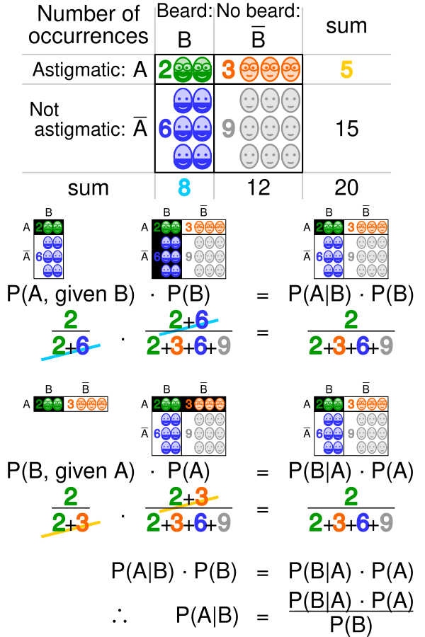
Probability theory basics

Top images from around the web for Probability theory basics

• 

  Bayesian inference - Wikipedia View original

  Is this image relevant?

• 

  Bayes' theorem - Wikipedia View original

  Is this image relevant?

• 

  Bayes’ Theorem | Mathematics for the Liberal Arts View original

  Is this image relevant?

• 

  Bayesian inference - Wikipedia View original

  Is this image relevant?

• 

  Bayes' theorem - Wikipedia View original

  Is this image relevant?

1 of 3

Top images from around the web for Probability theory basics

• 

  Bayesian inference - Wikipedia View original

  Is this image relevant?

• 

  Bayes' theorem - Wikipedia View original

  Is this image relevant?

• 

  Bayes’ Theorem | Mathematics for the Liberal Arts View original

  Is this image relevant?

• 

  Bayesian inference - Wikipedia View original

  Is this image relevant?

• 

  Bayes' theorem - Wikipedia View original

  Is this image relevant?

1 of 3

• Probability distributions describe the likelihood of different outcomes in random events
• Conditional probability quantifies the likelihood of an event given that another event has occurred
• Joint probability calculates the likelihood of two or more events occurring simultaneously
• Bayes' theorem relates conditional and marginal probabilities of events
• Law of total probability allows calculation of the probability of an event by considering all possible scenarios

Statistical inference concepts

• Population parameters represent true, unknown values in a population
• Sample statistics estimate population parameters based on observed data
• Estimators evaluate population parameters using mathematical functions of sample data
• Bias measures the difference between an estimator's expected value and the true parameter value
• Variance quantifies the spread of estimator values around its expected value
• Mean squared error combines bias and variance to assess estimator quality

Maximum likelihood principle

• Selects parameter values that maximize the probability of observing the given data
• Assumes the observed data is the most likely outcome under the chosen model
• Formulates a likelihood function to represent the joint probability of observations
• Identifies the parameter values that maximize the likelihood function
• Provides a systematic approach for parameter estimation in statistical models
• Applies to a wide range of probability distributions and model types

Maximum likelihood estimation

Likelihood function

• Mathematical expression representing the probability of observed data given model parameters
• Depends on both the data and the unknown parameters to be estimated
• Often denoted as $L(\theta|x)$ where $\theta$ represents parameters and $x$ represents data
• Constructed by multiplying individual probabilities of each observation
• Assumes independence between observations in many cases
• Can incorporate prior knowledge or constraints on parameter values

Log-likelihood function

• Logarithmic transformation of the likelihood function
• Simplifies calculations by converting products to sums
• Preserves the location of maximum points due to monotonicity of logarithm
• Denoted as $\ell(\theta|x) = \log L(\theta|x)$
• Improves numerical stability when dealing with very small probability values
• Allows for easier differentiation when finding maximum likelihood estimates

MLE vs other estimators

• Maximum likelihood estimators often have desirable statistical properties (consistency, efficiency)
• Method of moments estimators can be simpler to compute but may be less efficient
• Bayesian estimators incorporate prior information but require specification of prior distributions
• Least squares estimators minimize the sum of squared residuals between observed and predicted values
• Robust estimators perform well even when assumptions about the underlying distribution are violated
• Shrinkage estimators balance bias and variance to improve overall estimation accuracy

Applications in bioinformatics

Sequence alignment

• Estimates optimal alignment parameters (gap penalties, substitution scores) from observed sequence data
• Improves accuracy of pairwise and multiple sequence alignments
• Incorporates evolutionary models to account for sequence divergence over time
• Enables detection of conserved regions and functional motifs in protein or DNA sequences
• Facilitates homology detection and functional annotation of novel sequences

Phylogenetic tree reconstruction

• Infers evolutionary relationships between species or genes based on sequence data
• Estimates branch lengths and topology of phylogenetic trees
• Incorporates models of nucleotide or amino acid substitution
• Allows for testing of alternative evolutionary hypotheses
• Provides insights into speciation events and molecular clock calibration
• Supports comparative genomics and studies of gene family evolution

Gene finding algorithms

• Identifies coding regions and gene structures within genomic sequences
• Estimates parameters for splice site recognition, start and stop codon usage
• Incorporates species-specific codon usage bias and GC content
• Improves accuracy of gene prediction in newly sequenced genomes
• Facilitates annotation of complex gene structures (alternative splicing, overlapping genes)
• Supports comparative gene finding across multiple species

Computational aspects

Optimization techniques

• Gradient descent algorithms iteratively update parameters to maximize likelihood
• Newton-Raphson method uses second-order derivatives for faster convergence
• Quasi-Newton methods approximate second derivatives to reduce computational cost
• Coordinate descent optimizes parameters one at a time, useful for high-dimensional problems
• Stochastic gradient descent handles large datasets by using random subsets of data
• Conjugate gradient methods improve convergence in ill-conditioned optimization problems

Numerical methods

• Numerical integration approximates integrals when closed-form solutions are unavailable
• Root-finding algorithms locate zeros of likelihood equations
• Matrix decomposition techniques (LU, QR) solve systems of linear equations efficiently
• Interpolation methods estimate function values between known data points
• Finite difference methods approximate derivatives for optimization algorithms
• Adaptive quadrature adjusts integration step size based on function behavior

Software tools for MLE

• R packages (stats, bbmle) provide functions for maximum likelihood estimation
• Python libraries (scipy.optimize, statsmodels) offer MLE implementations
• MEGA software supports phylogenetic analysis using maximum likelihood methods
• PAML package specializes in phylogenetic analysis by maximum likelihood
• RAxML-NG enables high-performance phylogenetic tree inference
• IQ-TREE combines maximum likelihood with efficient tree search algorithms

Statistical properties

Consistency and efficiency

• Consistency ensures estimators converge to true parameter values as sample size increases
• Efficiency measures how close an estimator's variance is to the theoretical lower bound
• Maximum likelihood estimators are often asymptotically consistent and efficient
• Fisher information quantifies the amount of information data provides about parameters
• Cramér-Rao lower bound establishes a theoretical minimum variance for unbiased estimators
• Relative efficiency compares the performance of different estimators

Asymptotic normality

• Maximum likelihood estimators converge to a normal distribution as sample size increases
• Allows for approximation of sampling distributions for large samples
• Facilitates construction of confidence intervals and hypothesis tests
• Enables use of standard normal tables for inference about parameter estimates
• Asymptotic variance can be estimated using the observed Fisher information matrix
• Wald test utilizes asymptotic normality for hypothesis testing of parameter values

Confidence intervals

• Provide a range of plausible values for unknown parameters
• Constructed using the asymptotic normality property of maximum likelihood estimators
• Profile likelihood method adjusts for parameter interdependence in multidimensional problems
• Bootstrap resampling generates empirical distributions for parameter estimates
• Likelihood ratio test compares nested models to assess parameter significance
• Delta method approximates variance of transformed parameter estimates

Challenges and limitations

Model misspecification

• Incorrect assumptions about underlying probability distributions lead to biased estimates
• Omission of important variables or interactions affects model accuracy
• Overfitting occurs when models are too complex relative to available data
• Underfitting results from overly simplistic models that fail to capture important patterns
• Robust estimation techniques mitigate effects of outliers and departures from assumptions
• Model selection criteria (AIC, BIC) help balance model complexity and goodness-of-fit

Computational complexity

• High-dimensional parameter spaces increase computational demands
• Iterative optimization algorithms may converge slowly or get stuck in local optima
• Large datasets require efficient data structures and parallelization techniques
• Numerical instability can arise from ill-conditioned matrices or near-zero probabilities
• Approximation methods (variational inference, MCMC) handle complex likelihood functions
• GPU acceleration and distributed computing address computational bottlenecks

Small sample size issues

• Limited data leads to increased uncertainty in parameter estimates
• Bias correction techniques improve estimator performance for small samples
• Regularization methods prevent overfitting by adding constraints to parameter values
• Bayesian approaches incorporate prior information to stabilize estimates
• Jackknife and bootstrap resampling assess estimator variability with limited data
• Exact likelihood methods avoid asymptotic approximations for small sample inference

Advanced topics

Profile likelihood

• Focuses on a subset of parameters while treating others as nuisance parameters
• Reduces dimensionality of optimization problem by profiling out nuisance parameters
• Constructs confidence intervals that account for parameter interdependence
• Enables hypothesis testing for individual parameters in complex models
• Identifies practical non-identifiability in overparameterized models
• Visualizes likelihood surface to assess parameter uncertainty and correlations

Penalized maximum likelihood

• Adds penalty terms to likelihood function to encourage desired properties in estimates
• L1 regularization (Lasso) promotes sparsity by shrinking some coefficients to zero
• L2 regularization (Ridge) stabilizes estimates for highly correlated predictors
• Elastic net combines L1 and L2 penalties for improved variable selection
• Smoothing penalties enforce continuity or smoothness in function estimation
• Cross-validation selects optimal penalty strength to balance bias and variance

Expectation-maximization algorithm

• Iterative method for finding maximum likelihood estimates with incomplete data
• Alternates between expectation step (E-step) and maximization step (M-step)
• E-step computes expected value of log-likelihood given current parameter estimates
• M-step updates parameter estimates by maximizing the expected log-likelihood
• Handles missing data, latent variables, and mixture models efficiently
• Guarantees increase in likelihood at each iteration, ensuring convergence

Case studies in bioinformatics

Molecular evolution models

• Jukes-Cantor model assumes equal substitution rates between nucleotides
• Kimura two-parameter model distinguishes between transitions and transversions
• General time-reversible model allows for unequal base frequencies and substitution rates
• Codon substitution models incorporate selection pressure on protein-coding sequences
• Mixture models account for heterogeneity in evolutionary rates across sites
• Relaxed molecular clock models allow substitution rates to vary across lineages

Population genetics applications

• Estimates allele frequencies and genetic diversity within populations
• Infers demographic history (population size changes, migration) from genetic data
• Tests for deviations from Hardy-Weinberg equilibrium in genotype frequencies
• Detects signatures of natural selection in genomic regions
• Reconstructs haplotypes from unphased genotype data
• Estimates recombination rates and identifies recombination hotspots

Protein structure prediction

• Estimates parameters for energy functions in protein folding simulations
• Optimizes force field parameters to reproduce experimental structures
• Predicts secondary structure elements (alpha-helices, beta-sheets) from sequence data
• Estimates contact maps and distance restraints for tertiary structure modeling
• Refines homology models using maximum likelihood-based scoring functions
• Incorporates evolutionary information to improve structure prediction accuracy

Comparison with other methods

Maximum likelihood vs Bayesian inference

• Maximum likelihood provides point estimates, while Bayesian inference yields posterior distributions
• Bayesian methods incorporate prior knowledge through prior distributions on parameters
• Maximum likelihood often computationally simpler, especially for complex models
• Bayesian inference naturally handles uncertainty and allows for probabilistic predictions
• Maximum likelihood susceptible to overfitting in small samples, Bayesian methods can regularize
• Bayesian model averaging provides a framework for combining multiple models

Maximum likelihood vs parsimony

• Maximum likelihood incorporates explicit evolutionary models, parsimony minimizes changes
• Parsimony methods computationally faster but can be inconsistent under certain conditions
• Maximum likelihood accounts for multiple substitutions at the same site more effectively
• Parsimony performs well when substitution rates are low and sequences closely related
• Maximum likelihood provides natural framework for statistical hypothesis testing
• Parsimony methods do not require specification of substitution model parameters

Maximum likelihood vs distance methods

• Maximum likelihood uses all available sequence information, distance methods summarize as pairwise distances
• Distance methods computationally efficient for large datasets but may lose information
• Maximum likelihood handles missing data and alignment uncertainty more naturally
• Distance methods often used as starting points for more complex maximum likelihood analyses
• Maximum likelihood provides more accurate branch length estimates in phylogenetic trees
• Distance methods can be more robust to model misspecification in some cases

Future directions

Machine learning integration

• Deep learning approaches for parameter estimation in complex biological systems
• Neural networks as flexible function approximators in likelihood calculations
• Variational autoencoders for dimensionality reduction and generative modeling
• Reinforcement learning for optimizing experimental design in maximum likelihood estimation
• Transfer learning to leverage pre-trained models for related biological problems
• Interpretable machine learning techniques for understanding complex likelihood landscapes

Big data challenges

• Scalable algorithms for maximum likelihood estimation on massive genomic datasets
• Distributed computing frameworks (Spark, Dask) for parallel likelihood calculations
• Online learning methods for updating estimates as new data becomes available
• Approximate likelihood methods for intractable high-dimensional problems
• Dimension reduction techniques to focus on most informative features
• Privacy-preserving maximum likelihood estimation for sensitive biological data

Emerging applications in genomics

• Single-cell RNA-seq data analysis for cell type identification and lineage tracing
• Spatial transcriptomics for understanding gene expression patterns in tissue context
• Long-read sequencing data analysis for structural variant detection and haplotype phasing
• Multi-omics data integration for comprehensive understanding of biological systems
• Metagenomics and microbiome analysis for studying complex microbial communities
• Epigenomic data analysis for understanding gene regulation and chromatin structure