What is AP Physics 1 unit 7?
Oscillations appear whenever a restoring force pulls an object back toward equilibrium. Unit 7 formalizes that idea into simple harmonic motion, a model that applies to springs, pendulums, and many real systems. The unit builds from defining SHM, to calculating how fast a system oscillates, to representing the motion graphically, to tracking energy throughout the cycle.
Simple harmonic motion occurs when a restoring force is proportional to displacement from equilibrium. The key equations are m*a = -k*delta_x for the force condition, T = 2*pi*sqrt(m/k) for a spring, T = 2*pi*sqrt(L/g) for a pendulum, and E_total = (1/2)*k*A^2 for total mechanical energy. Kinetic energy is maximum at equilibrium; potential energy is maximum at the turning points.
What makes motion simple harmonic
SHM requires a linear restoring force: the net force on the object must point back toward equilibrium and be proportional to displacement. The equation m*a_x = -k*delta_x captures this. A pendulum with small angular displacement qualifies because the restoring torque is proportional to the angular displacement.
Period depends on system properties, not amplitude
For a spring-mass system, T = 2*pi*sqrt(m/k). For a simple pendulum, T = 2*pi*sqrt(L/g). Neither formula includes amplitude, which means doubling the amplitude of oscillation does not change how long each cycle takes. This is a frequently tested and counterintuitive result.
Energy shifts between kinetic and potential
Total mechanical energy in SHM is constant and equals (1/2)*k*A^2 for a spring system. At the turning points (x = plus or minus A), all energy is potential and kinetic energy is zero. At equilibrium (x = 0), all energy is kinetic and speed is maximum. Increasing amplitude increases total energy by a factor of A squared.
One framework, two systemsThe same SHM model describes both spring-mass oscillators and small-angle pendulums. In both cases a restoring force or torque is proportional to displacement, the period is amplitude-independent, and energy continuously converts between kinetic and potential forms while the total stays constant. Recognizing this shared structure lets you transfer reasoning from one system to the other on any problem.
Unit 7 review notes
7.1
The restoring force condition for SHM
SHM is a special case of periodic motion defined by its force law. The net force on the object must be a restoring force: it points opposite to the displacement from equilibrium and its magnitude is proportional to that displacement. The governing equation is m*a_x = -k*delta_x, where k is the spring constant and delta_x is displacement from equilibrium. Because acceleration is proportional to displacement and oppositely directed, the object accelerates most strongly at the turning points and has zero acceleration at equilibrium. A simple pendulum with small angular displacement fits this model because the restoring torque is proportional to the angular displacement, making the angular acceleration proportional to the angle.
- Restoring force: A force directed opposite to the object's displacement from equilibrium; its magnitude increases with displacement, pulling the object back.
- Equilibrium position: The location where net force on the object is zero; the object passes through this point with maximum speed.
- m*a_x = -k*delta_x: The defining SHM force equation; the negative sign confirms the force opposes displacement, and k sets how stiff the restoring force is.
- Small-angle approximation: For a pendulum, sin(theta) is approximately equal to theta in radians when the angle is small, making the restoring torque proportional to angular displacement and allowing the SHM model to apply.
A block on a spring is pulled 0.10 m from equilibrium and released. At what position is the net force on the block greatest in magnitude, and at what position is it zero?
| System | Restoring quantity | Proportionality condition |
|---|
| Spring-mass | Force F = -k*delta_x | Force proportional to linear displacement |
| Simple pendulum (small angle) | Torque tau proportional to theta | Torque proportional to angular displacement |
7.2
Calculating period and frequency for springs and pendulums
Period T and frequency f are inverses: T = 1/f. For a spring-mass system, T_s = 2*pi*sqrt(m/k). For a simple pendulum with small angular displacement, T_p = 2*pi*sqrt(L/g). Neither formula contains amplitude, confirming that amplitude does not affect how long each oscillation takes. To predict how a change in the system affects the period, isolate the variable that changed: doubling mass increases T_s by a factor of sqrt(2); quadrupling spring constant cuts T_s in half; doubling pendulum length increases T_p by sqrt(2); changing amplitude has no effect on either period.
- T = 1/f: Period and frequency are reciprocals; if a spring completes 2 oscillations per second, its period is 0.5 s.
- T_s = 2*pi*sqrt(m/k): Period of a spring-mass oscillator; increases with more mass and decreases with a stiffer spring.
- T_p = 2*pi*sqrt(L/g): Period of a simple pendulum; depends only on length and gravitational acceleration, not on the mass of the bob.
- Amplitude independence: For both the spring-mass system and the small-angle pendulum, the period is the same regardless of how large or small the oscillation is.
A pendulum has period T on Earth. If you take it to a planet where g is four times larger, what is the new period in terms of T?
| System | Period formula | Variables that change T | Variables that do NOT change T |
|---|
| Spring-mass | 2*pi*sqrt(m/k) | Mass m, spring constant k | Amplitude A |
| Simple pendulum | 2*pi*sqrt(L/g) | Length L, gravitational acceleration g | Bob mass, amplitude A |
7.3
Displacement, velocity, and acceleration graphs in SHM
Displacement in SHM follows x = A*cos(2*pi*f*t) or x = A*sin(2*pi*f*t) depending on initial conditions. Velocity and acceleration are also sinusoidal but shifted in phase. Velocity is zero at the turning points (x = plus or minus A) and maximum at equilibrium (x = 0). Acceleration is maximum in magnitude at the turning points and zero at equilibrium, always pointing opposite to displacement. On a graph, the x-t, v-t, and a-t curves all have the same period but peak at different times. Changing amplitude stretches the curves vertically but does not change the period or the horizontal spacing of the peaks and zeros.
- x = A*cos(2*pi*f*t): Displacement equation for an oscillator starting at maximum positive displacement; A is amplitude and f is frequency.
- Turning points: Positions x = plus or minus A where velocity is zero and acceleration (and restoring force) is maximum in magnitude.
- Equilibrium crossing: Position x = 0 where speed is maximum and acceleration is zero; the object passes through fastest here.
- Phase relationship: Velocity peaks one quarter cycle after displacement crosses zero; acceleration is always opposite in sign to displacement.
- Amplitude vs. period: Increasing amplitude raises the maximum values of displacement, velocity, and acceleration but leaves the period unchanged.
An object in SHM has displacement x = 0.05*cos(4*pi*t) meters. At t = 0, what are the displacement, velocity direction, and acceleration direction?
| Quantity | At x = +A (turning point) | At x = 0 (equilibrium) |
|---|
| Displacement | Maximum positive | Zero |
| Speed | Zero | Maximum |
| Acceleration magnitude | Maximum | Zero |
| Restoring force magnitude | Maximum | Zero |
7.4
Energy conservation in oscillating systems
The total mechanical energy of an SHM system is constant: E_total = U + K. For a spring-mass system, E_total = (1/2)*k*A^2. At the turning points, all energy is stored as spring potential energy U = (1/2)*k*x^2 and kinetic energy is zero. At equilibrium, all energy is kinetic and speed is at its maximum, v_max = A*sqrt(k/m). Because E_total scales with A squared, doubling the amplitude quadruples the total energy. This energy framework lets you find the speed of the object at any position using (1/2)*k*A^2 = (1/2)*m*v^2 + (1/2)*k*x^2.
- E_total = (1/2)*k*A^2: Total mechanical energy of a spring-mass oscillator; set by the amplitude and spring constant, not by position or time.
- U = (1/2)*k*x^2: Elastic potential energy at displacement x; maximum at the turning points and zero at equilibrium.
- K = (1/2)*m*v^2: Kinetic energy; maximum at equilibrium and zero at the turning points.
- v_max = A*sqrt(k/m): Maximum speed, reached when the object passes through equilibrium; increases with amplitude and decreases with more mass.
- Energy and amplitude: Total energy is proportional to A squared, so a larger amplitude means more total energy stored in the system.
A spring with k = 200 N/m oscillates with amplitude 0.04 m. What is the total mechanical energy, and what is the speed of the mass at x = 0.02 m if the mass is 0.5 kg?
| Position | Kinetic energy | Potential energy | Total energy |
|---|
| x = A (turning point) | Zero | Maximum = (1/2)*k*A^2 | (1/2)*k*A^2 |
| x = 0 (equilibrium) | Maximum = (1/2)*k*A^2 | Zero | (1/2)*k*A^2 |
| x between 0 and A | Partial | Partial | (1/2)*k*A^2 |
Practice AP Physics 1 unit 7 questions
Try stimulus-based AP practice questions and written prompts after you review the notes.
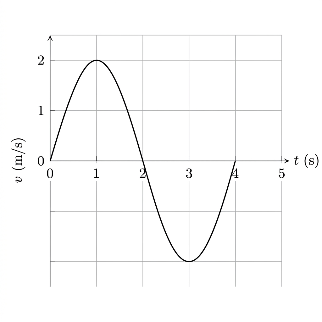
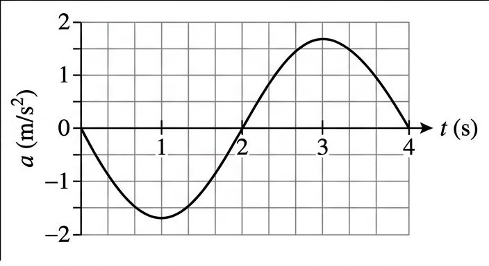
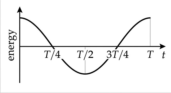
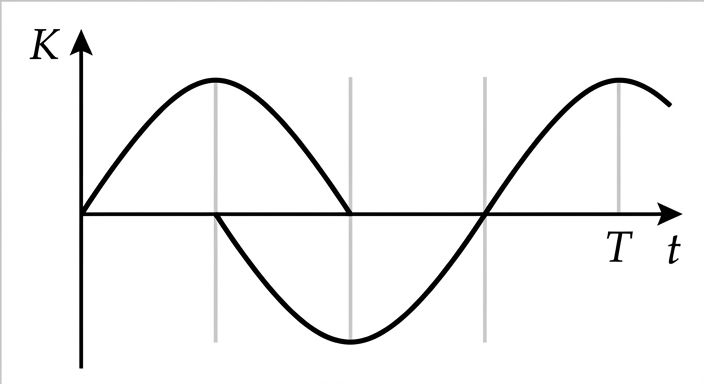
A simple pendulum oscillates with a small amplitude. The graph shows the horizontal velocity v of the pendulum bob as a function of time t.
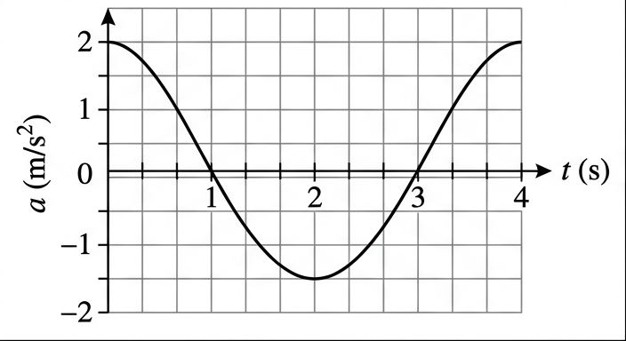
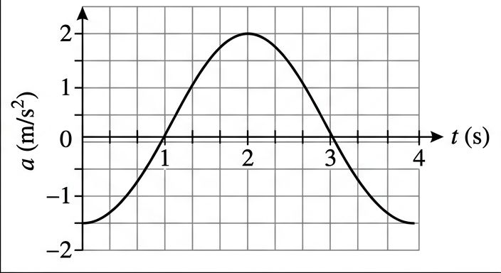
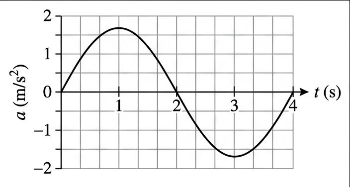
QuestionWhich of the following graphs could represent the horizontal acceleration a of the pendulum bob as a function of time t?
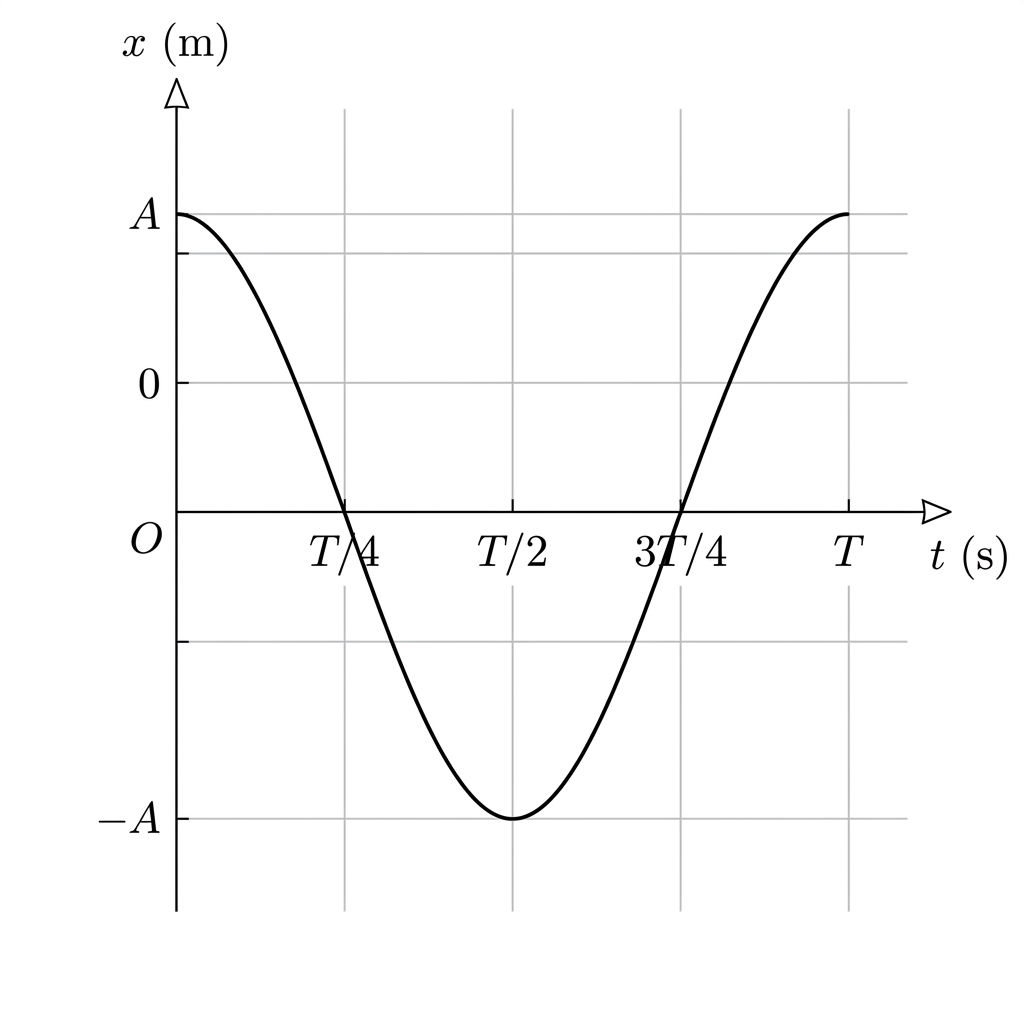
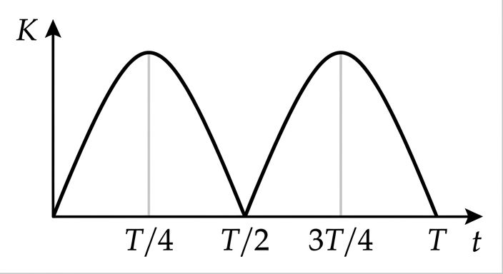
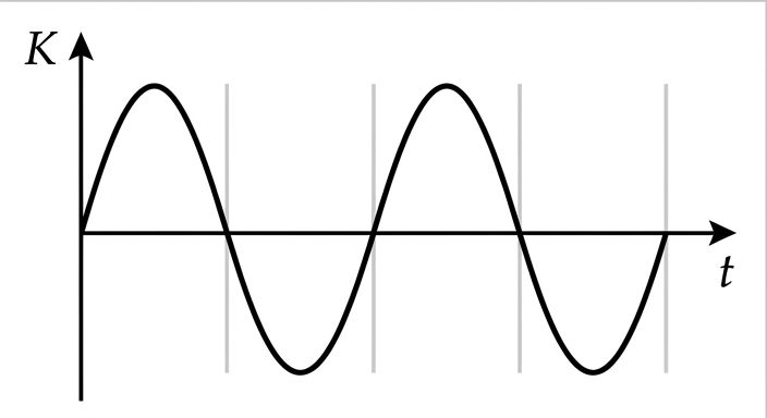
A block attached to a horizontal spring oscillates on a frictionless surface. The graph shows the block's position x as a function of time t.
QuestionWhich of the following graphs could represent the kinetic energy K of the block as a function of time t?
2. A cart of mass 0.50 kg (see Figure 1) is attached to a spring and oscillates on a horizontal, frictionless track.
Figure 1. Cart–spring system at three specific positions: +0.20 m (released from rest), 0 m (equilibrium), and −0.20 m (turning point).
Figure 2. Energy bar chart at x = +0.20 m (released from rest).
Figure 3. Energy bar chart at x = 0 m (equilibrium).
Figure 4. Reference energy bar chart at x = −0.10 m (provides the energy scale).
• Shaded bars should start at the dashed line that represents zero energy.
• Represent any energy that is equal to zero with a distinct line on the zero-energy line.
• The relative heights of each shaded bar should reflect the magnitude of the respective energy consistent with the scale used in Figure 4.
Figure 5. Cart at x = +0.20 m released from rest, and at x = 0 m moving with maximum speed v_max.
Figure 6. Energy vs. position for the cart–spring system from x = −0.20 m to x = +0.20 m, with Uₛ(x) given; students add E and K(x).
i. Sketch and label a line that represents the total mechanical energy E for the cart-spring system as a function of the position x from x=−0.20 m to x=+0.20 m.
ii. Sketch and label a curve that represents the kinetic energy K(x) for the cart-spring system as a function of the position x from x=−0.20 m to x=+0.20 m.
∣a0.10∣>∣a0.20∣
∣a0.10∣<∣a0.20∣
∣a0.10∣=∣a0.20∣
Justify how your response is consistent with the energy lines or curves you drew in Figure 6 in part C.
4. In Scenario 1, a block of mass m1=0.60 kg is attached to a horizontal ideal spring with spring constant k=120 N/m on a frictionless surface, as shown in Figure 1. The block is pulled to the right to a displacement x=+0.10 m from equilibrium and released from rest. The block subsequently undergoes simple harmonic motion. All frictional forces are negligible.
In Scenario 2, the spring is attached to a different block of mass m2=0.90 kg on the same frictionless surface, as shown in Figure 2. The block is again pulled to the right to the same displacement x=+0.10 m from equilibrium and released from rest. The block subsequently undergoes simple harmonic motion. All frictional forces are negligible.
Figure 1. Scenario 1: Block–spring system on a frictionless horizontal surface, with the block pulled to x = +0.10 m and released.
Figure 2. Scenario 2: Same block–spring setup, but with mass m₂ = 0.90 kg; block pulled to the same displacement x = +0.10 m.
• a1>a2
• a1<a2
• a1=a2
Justify your answer in terms of ALL forces exerted on the block at the instant it is released in each scenario. Use qualitative reasoning beyond referencing equations.
1. A student investigates the horizontal motion of a block attached to a spring on a frictionless horizontal surface, as shown in Figure 1. The block is attached to the spring, which is fixed to a wall. The block is displaced from equilibrium and released, undergoing simple harmonic motion (SHM).
Figure 1. Block–spring system on a frictionless horizontal surface at the instant of release.
Figure 2. Axes for a position–time graph x versus t over one full period T.
i. On the axes shown in Figure 2, sketch a graph of the position x of the block as a function of time t for one full period from t = 0 to t = T. Be sure to indicate the values of x at t = 0, t = T/4, t = T/2, and t = T.
ii. Derive an expression for the period T of the oscillations in terms of the mass m and the spring constant k. Begin your derivation by writing a fundamental physics principle or an equation from the reference information.
iii. Derive an expression for the maximum speed v_max of the block in terms of the amplitude A, the mass m, and the spring constant k. Begin your derivation by writing a fundamental physics principle or an equation from the reference information.
Increases
Decreases
Remains the same
Justify your response.