Joint, marginal, and conditional distributions are key concepts in probability theory. They help us understand relationships between multiple random variables, allowing us to calculate probabilities and make predictions in complex scenarios.

These distributions are crucial for analyzing real-world situations in fields like finance, medicine, and engineering. By mastering them, you'll be able to tackle advanced problems involving multiple variables and make informed decisions based on probabilistic models.

Joint, Marginal, and Conditional Distributions

Defining and Interpreting Distributions

Top images from around the web for Defining and Interpreting Distributions
  • A joint probability distribution gives the probability of each possible outcome for two or more random variables
  • The (PMF) for discrete random variables X and Y, denoted as , gives the probability that X takes on the value x and Y takes on the value y simultaneously
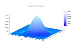
  • The (PDF) for continuous random variables X and Y, denoted as , gives the probability density at the point (x, y) in the XY-plane
  • A marginal probability distribution is derived from a by summing or integrating the joint probabilities over the other random variable(s)
    • The marginal PMF for a discrete random variable X is calculated as = _y P(X=x, Y=y), where the sum is taken over all possible values of Y
    • The marginal PDF for a continuous random variable X is calculated as f_X(x) = _(-∞)^∞ f(x, y) dy, where the integral is taken over the entire range of Y
  • A conditional probability distribution is a probability distribution of one random variable given the value or range of values of another random variable
    • The conditional PMF for discrete random variables X and Y, denoted as , gives the probability that Y takes on the value y given that X takes on the value x
    • The conditional PDF for continuous random variables X and Y, denoted as f(y | x), gives the probability density of Y at the point y given that X takes on the value x

Examples of Joint, Marginal, and Conditional Distributions

  • Joint distribution example: The joint PMF of the number of defective items (X) and the number of non-defective items (Y) in a sample of 10 items from a production line
  • example: The marginal PMF of the number of defective items (X) in the sample, calculated by summing the joint probabilities over all possible values of Y
  • example: The conditional PMF of the number of non-defective items (Y) given that there are 2 defective items (X=2) in the sample
  • Joint PDF example: The joint PDF of the height (X) and weight (Y) of adult males in a population
  • Marginal PDF example: The marginal PDF of the height (X) of adult males, obtained by integrating the joint PDF over the entire range of weights (Y)
  • Conditional PDF example: The conditional PDF of the weight (Y) of adult males given a height (X) of 180 cm

Probability Calculations with Multiple Variables
Calculating Probabilities, Expected Values, and Variances

  • Probabilities for events involving multiple random variables can be calculated using joint, marginal, and conditional distributions
    • For discrete random variables, P(X=x, Y=y) = P(X=x)P(Y=y | X=x) = by the multiplication rule of probability
    • For continuous random variables, P(a ≤ X ≤ b, c ≤ Y ≤ d) = ∫_a^b ∫_c^d f(x, y) dy dx, where the double integral is taken over the specified ranges of X and Y
  • The (mean) of a function g(X, Y) of two random variables X and Y is calculated as:
    • E[g(X, Y)] = Σ_x Σ_y g(x, y)P(X=x, Y=y) for discrete random variables
    • E[g(X, Y)] = ∫(-∞)^∞ ∫(-∞)^∞ g(x, y)f(x, y) dy dx for continuous random variables
  • The expected value of X can be calculated using the marginal PMF or PDF of X: E[X] = Σ_x xP(X=x) for discrete X and E[X] = ∫_(-∞)^∞ xf_X(x) dx for continuous X
  • The conditional expected value of Y given X=x is calculated as E[Y | X=x] = Σ_y yP(Y=y | X=x) for discrete Y and E[Y | X=x] = ∫_(-∞)^∞ yf(y | x) dy for continuous Y
  • The of a function g(X, Y) of two random variables X and Y is calculated as Var[g(X, Y)] = E[g(X, Y)^2] - (E[g(X, Y)])^2, where the expected values are calculated using the joint distribution of X and Y
    • The variance of X can be calculated using the marginal PMF or PDF of X: Var[X] = E[X^2] - (E[X])^2
    • The conditional variance of Y given X=x is calculated as Var[Y | X=x] = E[Y^2 | X=x] - (E[Y | X=x])^2, where the conditional expected values are used

Examples of Probability Calculations

  • Joint probability example: Calculate the probability that a randomly selected adult male has a height between 170 cm and 180 cm and a weight between 70 kg and 80 kg, given the joint PDF of height and weight
  • Marginal probability example: Calculate the probability that a randomly selected item from a production line is defective, using the marginal PMF of the number of defective items in a sample
  • Conditional probability example: Calculate the probability that a patient has a disease given the presence of a specific symptom, using the conditional PMF of the disease status given the symptom status
  • Expected value example: Calculate the expected total cost of a project with two components, given the joint PMF of the costs of each component
  • Variance example: Calculate the variance of the total number of items sold by two salespeople, given the joint PMF of the number of items sold by each salesperson

Independence of Random Variables
Determining Independence Using Joint and Marginal Distributions

  • Two random variables X and Y are independent if and only if their joint probability distribution is equal to the product of their marginal distributions for all possible values of X and Y
    • For discrete random variables, X and Y are independent if and only if P(X=x, Y=y) = P(X=x)P(Y=y) for all x and y
    • For continuous random variables, X and Y are independent if and only if f(x, y) = f_X(x)f_Y(y) for all x and y
  • If X and Y are independent, then knowing the value of one variable does not provide any information about the value of the other variable
  • When X and Y are independent, the conditional probability distribution of Y given X=x is equal to the marginal distribution of Y for all x, and vice versa
    • For discrete random variables, if X and Y are independent, then P(Y=y | X=x) = P(Y=y) for all x and y
    • For continuous random variables, if X and Y are independent, then f(y | x) = f_Y(y) for all x and y
  • The correlation coefficient ρ between two independent random variables is always equal to zero, but a correlation of zero does not necessarily imply independence

Examples of Independence and Dependence

  • Independent discrete random variables example: The outcomes of two fair dice rolls are independent, as the probability of any outcome on the second roll is not affected by the outcome of the first roll
  • Independent continuous random variables example: The heights of two randomly selected individuals from a population are independent, as the height of one person does not influence the height of another person
  • Dependent discrete random variables example: The number of defective items and the number of non-defective items in a sample from a production line are dependent, as the total number of items in the sample is fixed
  • Dependent continuous random variables example: The weight and body mass index (BMI) of an individual are dependent, as BMI is calculated using both weight and height

Applications of Joint Distributions

Modeling and Analyzing Real-World Situations

  • Joint, marginal, and conditional distributions can be used to model and analyze real-world situations involving multiple random variables, such as:
    • Quality control: The joint distribution of the lengths and widths of manufactured parts can be used to determine the probability of a part meeting specifications
    • Medical diagnosis: The joint distribution of the presence or absence of various symptoms can be used to calculate the probability of a patient having a specific disease
    • Finance: The joint distribution of the returns on two or more assets can be used to assess the risk and potential returns of an investment portfolio
  • When solving problems involving multiple random variables, it is essential to identify the relevant joint, marginal, and conditional distributions and use them to calculate the desired probabilities, expected values, or variances
  • In some cases, it may be necessary to derive the required distributions from the given information or assumptions about the random variables and their relationships
  • When working with conditional distributions, it is crucial to correctly identify the conditioning event and use the appropriate probability rules, such as , to calculate the desired probabilities or expected values
  • Independence assumptions can simplify calculations and problem-solving, but it is essential to verify that the random variables are indeed independent before applying these simplifications

Examples of Applications

  • Quality control example: A manufacturer wants to determine the probability that a randomly selected product meets the length and width specifications, given the joint PDF of the length and width of the products
  • Medical diagnosis example: A doctor wants to calculate the probability that a patient has a rare disease, given the presence of two specific symptoms and the joint PMF of the disease status and symptom statuses
  • Finance example: An investor wants to find the optimal allocation of funds between two stocks to maximize the expected return while keeping the variance of the portfolio below a certain threshold, using the joint PDF of the stock returns
  • Marketing example: A company wants to estimate the expected total sales of two products based on the joint PMF of the number of units sold for each product during a promotional event
  • Insurance example: An insurance company wants to determine the probability that the total claim amount from two policyholders exceeds a certain value, given the joint PDF of the claim amounts for each policyholder

Key Terms to Review (29)

: The symbol ∫ represents the integral in calculus, which is a fundamental concept used to compute the area under a curve or to determine the accumulation of quantities. It connects deeply with joint, marginal, and conditional distributions by allowing us to find probabilities over specified intervals in continuous random variables. Integrals are essential for transitioning from discrete to continuous distributions, helping to understand relationships and dependencies between random variables.
Bayes' Theorem: Bayes' Theorem is a mathematical formula used to update the probability of a hypothesis based on new evidence. It establishes a relationship between joint, marginal, and conditional probabilities, allowing us to make informed decisions by revising our beliefs when presented with new data. This theorem plays a crucial role in understanding how prior beliefs and new information interact, especially in Bayesian inference, where it is used to derive posterior distributions from prior distributions and observed data.
Bayesian inference: Bayesian inference is a statistical method that applies Bayes' theorem to update the probability of a hypothesis as more evidence or information becomes available. This approach emphasizes the importance of prior beliefs and knowledge, allowing for a systematic way to incorporate new data and refine predictions. The process involves calculating the posterior distribution, which combines prior distributions and likelihoods, enabling a coherent interpretation of uncertainty in the presence of incomplete information.
Conditional Distribution: Conditional distribution is the probability distribution of a random variable given that another random variable takes on a specific value. This concept is crucial for understanding how two variables interact with each other and helps identify relationships between them, particularly in the context of joint and marginal distributions, where you can analyze how the distribution of one variable changes based on the value of another.
Conditional Independence: Conditional independence refers to a statistical property where two random variables are independent of each other given the value of a third variable. This means that once you know the value of the third variable, knowing the value of one of the other variables does not provide any additional information about the other variable. This concept plays a significant role in understanding joint, marginal, and conditional distributions, as it helps to simplify complex probability models by reducing the number of dependencies among variables.
Conditional Probability Density Function: A conditional probability density function describes the likelihood of a random variable taking on a specific value given that another related variable has a known value. It is a key concept in understanding how variables interact with one another, allowing us to analyze relationships and dependencies within joint distributions. This function helps in isolating the effects of one variable on another, making it essential for statistical modeling and inference.
Conditional Probability Mass Function: A conditional probability mass function (PMF) defines the probability distribution of a discrete random variable given that another random variable takes on a specific value. It allows us to understand how one variable behaves under the condition that we know something about another variable, linking directly to joint distributions and marginal distributions.
Contingency Tables: Contingency tables are a type of table used in statistics to display the frequency distribution of variables, allowing researchers to analyze the relationship between two categorical variables. They summarize the joint distribution of data points in a matrix format, where rows typically represent one variable and columns represent another. This organization helps in understanding joint, marginal, and conditional distributions effectively.
Covariance: Covariance is a statistical measure that indicates the extent to which two random variables change together. If the variables tend to increase and decrease in tandem, the covariance is positive; if one variable increases while the other decreases, the covariance is negative. This concept is crucial when analyzing joint, marginal, and conditional distributions, as it helps in understanding relationships between variables within these distributions.
Expected Value: Expected value is a fundamental concept in probability and statistics that represents the average outcome of a random variable, weighted by the probabilities of each outcome occurring. It provides a measure of the center of a probability distribution and is crucial for understanding the behavior of random variables in various scenarios, whether independent or dependent. This concept connects to joint, marginal, and conditional distributions as it helps analyze multi-dimensional random variables, and it plays a key role in moment generating functions for deriving important characteristics of those distributions.
F(x, y): The notation f(x, y) represents a joint probability distribution function for two random variables, x and y. This function provides the likelihood of various outcomes occurring together for the two variables, allowing us to analyze the relationship and dependence between them. By understanding f(x, y), one can also derive marginal and conditional distributions, which break down the joint distribution into simpler components.
Independent Events: Independent events are occurrences in probability where the outcome of one event does not affect the outcome of another. This concept is crucial in understanding how probabilities combine, as it allows for the multiplication of individual probabilities to find the likelihood of multiple events happening together without influence from each other.
Joint distribution: Joint distribution refers to the probability distribution that captures the likelihood of two or more random variables occurring simultaneously. It provides a comprehensive view of the relationship between these variables, revealing how their values interact with each other, which is crucial for understanding joint, marginal, and conditional distributions.
Joint probability density function: A joint probability density function (PDF) is a mathematical function that describes the likelihood of two or more continuous random variables occurring simultaneously. It provides a way to understand how different variables are related and the probability of specific outcomes across multiple dimensions. This concept is vital for understanding joint, marginal, and conditional distributions, as it lays the foundation for calculating probabilities involving multiple variables.
Joint probability mass function: A joint probability mass function (PMF) is a function that gives the probability that two discrete random variables take on specific values simultaneously. It captures the relationship between the variables, showing how the likelihood of one variable occurring depends on the other. Understanding the joint PMF helps in analyzing and interpreting the behavior of multiple random variables together, leading to insights about marginal and conditional distributions.
Law of Total Probability: The law of total probability states that the probability of an event can be found by considering all possible ways that event can occur, weighted by the probabilities of each scenario. This concept is particularly important when dealing with joint, marginal, and conditional distributions, as it provides a way to relate these different types of probabilities and helps in calculating probabilities when conditional probabilities and marginal probabilities are involved.
Marginal Distribution: Marginal distribution refers to the probability distribution of a subset of variables within a joint distribution, focusing on a single variable while ignoring the others. It provides insight into the behavior and characteristics of one variable across all possible values of the other variables in the dataset. This is important for understanding how each variable contributes to the overall joint distribution and is often used in conjunction with conditional distributions to analyze relationships between variables.
Marginal Probability Mass Function: The marginal probability mass function (PMF) describes the probability distribution of a single discrete random variable, regardless of the values of other variables in a joint distribution. It is derived by summing or integrating the joint probabilities over the other variables, allowing us to focus on one variable's behavior without considering the influence of others. This concept connects directly to joint and conditional distributions, as it provides a way to isolate individual probabilities from a multi-dimensional context.
Maximum Likelihood Estimation: Maximum likelihood estimation (MLE) is a statistical method used to estimate the parameters of a probabilistic model by maximizing the likelihood function, which measures how well the model explains the observed data. This technique relies on the concept of joint, marginal, and conditional distributions, where MLE seeks to find the parameter values that make the observed data most probable. By applying MLE, one can derive estimates in various statistical contexts, such as logistic regression, factor analysis, structural equation modeling, and point estimation.
P(x=x | y=y): The notation p(x=x | y=y) represents the conditional probability of a random variable X taking a specific value x, given that another random variable Y has taken a specific value y. This concept is crucial in understanding how the occurrence of one event can influence the probability of another event, highlighting the relationship between joint distributions and conditional distributions in statistics.
P(x=x, y=y): p(x=x, y=y) represents the joint probability distribution of two discrete random variables X and Y, indicating the likelihood of both X taking the value x and Y taking the value y simultaneously. This concept is essential for understanding relationships between multiple variables, as it provides a way to assess how likely certain outcomes are when considering more than one variable together. Joint probabilities help us understand how two events are related or dependent on each other.
P(x=x): The notation p(x=x) refers to the probability that a random variable X takes on a specific value x. This concept is central to understanding how probabilities are distributed among different outcomes, linking to ideas of joint, marginal, and conditional distributions. By analyzing p(x=x), one can derive insights into the behavior of random variables in various scenarios and how they relate to one another within a statistical framework.
P(y=y | x=x): The expression p(y=y | x=x) refers to the conditional probability of the event Y taking on a specific value y, given that another variable X is equal to a particular value x. This concept plays a crucial role in understanding the relationships between variables and is essential for exploring joint, marginal, and conditional distributions in probability theory.
P(y=y): The term p(y=y) represents the probability that a random variable Y takes on a specific value y, which can be interpreted in the context of joint, marginal, and conditional distributions. This notation reflects the likelihood of observing the value y within the probability distribution of Y, and it can be crucial for understanding how different variables relate to each other in multivariate scenarios. This concept connects to how we analyze relationships between multiple variables and how to quantify those relationships through probability distributions.
Probability Density Function: A probability density function (PDF) describes the likelihood of a continuous random variable taking on a particular value. Unlike discrete distributions, which use probability mass functions, a PDF assigns probabilities to intervals of values rather than individual outcomes. The area under the curve of a PDF represents the total probability of all possible values, and the function must satisfy certain properties, such as being non-negative and integrating to one over its entire range.
Probability Tables: Probability tables are systematic representations that display the likelihood of different outcomes in a probabilistic scenario. They provide a structured way to view joint, marginal, and conditional probabilities, making it easier to analyze relationships between multiple variables and understand how probabilities change based on specific conditions.
Scatter plot: A scatter plot is a type of data visualization that displays values for two variables using Cartesian coordinates. Each point on the graph represents an observation from a dataset, showing how one variable is affected by another. By examining the pattern of the points, one can identify relationships, trends, or correlations between the two variables, which connects to understanding joint, marginal, and conditional distributions as well as the types of data and variables involved in the analysis.
Variance: Variance is a statistical measure that quantifies the degree of spread or dispersion of a set of values in a dataset. It helps to understand how much the individual data points differ from the mean value, which is crucial for evaluating the consistency and reliability of data in various contexts.
σ: In statistics, σ (sigma) represents the standard deviation, which measures the amount of variation or dispersion of a set of values. A low σ indicates that the values tend to be close to the mean, while a high σ indicates that the values are spread out over a wider range. Understanding σ is crucial when analyzing joint, marginal, and conditional distributions, as it helps in understanding the relationships and variability among different variables.
© 2024 Fiveable Inc. All rights reserved.
AP® and SAT® are trademarks registered by the College Board, which is not affiliated with, and does not endorse this website.