Matrix polynomials are powerful tools in advanced linear algebra. They're like regular polynomials, but with matrices as variables. This means we can do cool stuff like solve complex equations and analyze systems in ways that weren't possible before.

Evaluating these polynomials can be tricky, but there are smart methods to make it easier. We'll look at different techniques, from basic calculations to fancy eigendecomposition approaches. These skills are super useful in real-world applications like signal processing and network analysis.

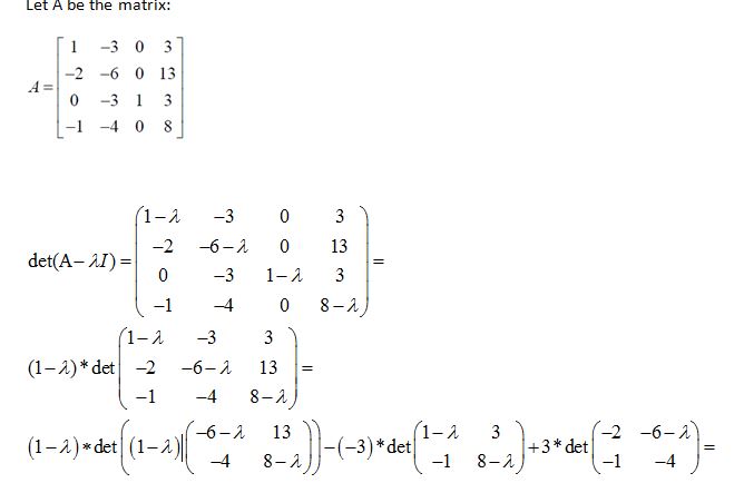
Matrix Polynomials and Their Properties

Definition and Structure

Top images from around the web for Definition and Structure
  • Matrix polynomials consist of polynomial expressions with square matrix variables and scalar or compatible matrix coefficients
  • General form: [P(A)](https://www.fiveableKeyTerm:p(a))=anAn+an1An1+...+a1A+a0I[P(A)](https://www.fiveableKeyTerm:p(a)) = a_n A^n + a_{n-1} A^{n-1} + ... + a_1 A + a_0 I
    • A represents a square matrix
    • a_i denotes scalar coefficients
    • I stands for the identity matrix
  • Degree determined by the highest power of the matrix variable in the expression
  • Closed under addition and multiplication
    • Sum or product of two matrix polynomials yields another
  • Form a ring with zero polynomial and identity matrix as additive and multiplicative identities

Algebraic Properties

  • Follow similar properties as scalar polynomials (addition, multiplication, composition)
  • Addition of matrix polynomials
    • P(A)+Q(A)=(an+bn)An+(an1+bn1)An1+...+(a0+b0)IP(A) + Q(A) = (a_n + b_n)A^n + (a_{n-1} + b_{n-1})A^{n-1} + ... + (a_0 + b_0)I
  • Multiplication of matrix polynomials
    • (PQ)(A)=i=0mj=0naibjAi+j(P \cdot Q)(A) = \sum_{i=0}^m \sum_{j=0}^n a_i b_j A^{i+j}
  • Composition of matrix polynomials
    • (PQ)(A)=P(Q(A))(P \circ Q)(A) = P(Q(A))

Applications and Significance

  • Crucial in solving differential equations (linear systems, control theory)
  • Utilized in signal processing (digital filter design, frequency response analysis)
  • Applied in control theory (stability analysis, feedback systems)
  • Employed in network analysis (centrality measures, graph spectra)

Evaluating Matrix Polynomials

Direct Computation and Horner's Method

  • Direct computation involves evaluating each term separately and summing results
    • Follow matrix arithmetic order of operations
  • rewrites the polynomial in nested form
    • Minimizes required matrix multiplications
    • P(A)=(...((anA+an1)A+an2)A+...+a1)A+a0IP(A) = (...((a_n A + a_{n-1})A + a_{n-2})A + ... + a_1)A + a_0 I

Eigendecomposition and Taylor Series Methods

  • Eigendecomposition method diagonalizes matrix A as A=PDP1A = PDP^{-1}
    • D represents a diagonal matrix of eigenvalues
    • Evaluate using P(A)=PP(D)P1P(A) = PP(D)P^{-1}
  • Taylor series expansion approximates matrix polynomials
    • Truncate series around a suitable point
    • P(A)P(A0)+P(A0)(AA0)+12!P(A0)(AA0)2+...P(A) \approx P(A_0) + P'(A_0)(A - A_0) + \frac{1}{2!}P''(A_0)(A - A_0)^2 + ...

Advanced Techniques

  • Cayley-Hamilton theorem simplifies higher degree polynomial evaluations
    • Every matrix satisfies its own characteristic polynomial
  • Krylov subspace methods efficiently approximate evaluations for large sparse matrices
    • Utilize iterative techniques based on Krylov subspaces
  • Interpolation-based methods employ matrix interpolation techniques
    • Especially effective for matrices with clustered eigenvalues

Applications of Matrix Polynomials

Solving Matrix Equations

  • Essential in solving linear systems P(A)x=bP(A)x = b
    • P(A) represents a matrix polynomial
  • Compute matrix functions through polynomial expansions
    • Matrix exponential: eAI+A+12!A2+13!A3+...e^A \approx I + A + \frac{1}{2!}A^2 + \frac{1}{3!}A^3 + ...
    • Matrix sine: sin(A)A13!A3+15!A5...\sin(A) \approx A - \frac{1}{3!}A^3 + \frac{1}{5!}A^5 - ...
  • Find matrix inverse using Cayley-Hamilton theorem and adjugate matrix method
    • A1=1an(an1I+an2A+...+An1)A^{-1} = -\frac{1}{a_n}(a_{n-1}I + a_{n-2}A + ... + A^{n-1})

Dynamical Systems and Signal Processing

  • Analyze stability in dynamical systems
    • Characteristic polynomial of system matrix determines stability properties
  • Design digital filters and analyze frequency responses
    • Transfer functions represented as matrix polynomials
  • Study Markov chains and stochastic processes
    • Analyze long-term behavior and steady-state distributions
    • Pn=limnP(A)nP^n = \text{lim}_{n \to \infty} P(A)^n

Network and Graph Analysis

  • Compute centrality measures in complex networks
    • Eigenvector centrality: Ax=λxAx = \lambda x
  • Analyze graph spectra and structural properties
    • Adjacency matrix polynomials reveal path counts and connectivity

Matrix Polynomials vs Matrix Exponential

Series Expansion and Approximation

  • Matrix exponential defined as limit of matrix polynomial series
    • exp(A)=I+A+12!A2+13!A3+...\exp(A) = I + A + \frac{1}{2!}A^2 + \frac{1}{3!}A^3 + ...
  • Truncating series results in matrix polynomial approximation
    • Higher-order terms improve accuracy
    • exp(A)I+A+12!A2+...+1n!An\exp(A) \approx I + A + \frac{1}{2!}A^2 + ... + \frac{1}{n!}A^n

Efficient Computation Methods

  • Padé approximation provides rational function approximation
    • More efficient than direct series expansion
    • exp(A)Pm(A)Qn(A)\exp(A) \approx \frac{P_m(A)}{Q_n(A)}
  • Scaling and squaring techniques combined with polynomial evaluation
    • Efficient for large matrices
    • exp(A)=[exp(A/2k)]2k\exp(A) = [\exp(A/2^k)]^{2^k}

Properties and Applications

  • Fundamental property: exp(A+B)=exp(A)exp(B)\exp(A + B) = \exp(A)\exp(B) when A and B commute
  • Crucial in solving systems of linear differential equations
    • ddtx(t)=Ax(t)\frac{d}{dt}x(t) = Ax(t) has solution x(t)=exp(At)x(0)x(t) = \exp(At)x(0)
  • Connection extends to other matrix functions
    • Matrix logarithm: log(I+A)=A12A2+13A3...\log(I + A) = A - \frac{1}{2}A^2 + \frac{1}{3}A^3 - ...
    • Matrix sine: sin(A)=A13!A3+15!A5...\sin(A) = A - \frac{1}{3!}A^3 + \frac{1}{5!}A^5 - ...

Key Terms to Review (18)

A^k: In the context of matrix polynomial evaluation, 'a^k' represents the k-th power of a matrix 'A'. This operation involves multiplying the matrix by itself 'k' times, which is fundamental in calculating matrix functions and evaluating polynomials where matrices are involved. This concept is critical for understanding how matrices behave under exponentiation and is widely used in various applications, including solving systems of linear equations and in control theory.
Associativity: Associativity refers to the property of certain operations where the grouping of operands does not affect the result. This means that when performing an operation on multiple elements, the way in which the elements are grouped can be changed without altering the outcome. Understanding associativity is crucial when evaluating expressions involving matrices and tensors, as it allows for flexibility in computation, especially with complex operations like matrix polynomials and tensor products.
Cauchy-like integrals: Cauchy-like integrals are integral expressions used to evaluate matrix polynomials by leveraging properties of complex analysis and residue calculus. These integrals take a specific form that allows for the evaluation of matrix functions through contour integration, which can simplify the computation of polynomials in matrices, particularly when the matrices have complex eigenvalues. This technique is often crucial for obtaining results in numerical linear algebra and spectral theory.
Direct substitution: Direct substitution is a method used to evaluate matrix polynomials by substituting specific matrices into the polynomial expression. This process allows one to compute the value of the polynomial for a given matrix by replacing the variable with the matrix itself, enabling straightforward calculations and insights into the polynomial's behavior.
Distributivity: Distributivity refers to the algebraic property that allows multiplication to be distributed over addition or subtraction. This means that for any elements a, b, and c, the equation a imes (b + c) = a imes b + a imes c holds true. This property is crucial for simplifying expressions and solving equations involving matrices and tensors, helping to break down complex operations into more manageable parts.
Eigenvalue decomposition: Eigenvalue decomposition is a mathematical technique where a matrix is expressed in terms of its eigenvalues and eigenvectors. This process allows a square matrix to be factored into a set of eigenvalues that represent the scaling factors and eigenvectors that indicate the directions in which the transformations occur. It is crucial for understanding properties of matrices, particularly in solving linear systems and performing dimensionality reduction techniques.
Evaluation at a point: Evaluation at a point refers to the process of substituting a specific value into a matrix polynomial to obtain a resulting matrix. This operation is essential in understanding how matrix polynomials behave when applied to particular values, allowing us to analyze their properties and apply them in various mathematical contexts. This concept plays a crucial role in matrix computations, as it provides insights into the dynamics and transformations represented by the polynomial when evaluated at a given matrix.
Horner's Method: Horner's Method is an efficient algorithm used for the evaluation of polynomial expressions, especially useful in the context of numerical computations. This method rewrites a polynomial in a nested form, which minimizes the number of multiplications and additions required for its evaluation. By structuring the polynomial in this way, it not only simplifies calculations but also enhances numerical stability when working with matrices and polynomials.
Image processing: Image processing refers to the technique of manipulating and analyzing digital images through algorithms and mathematical operations. This process is crucial in enhancing image quality, extracting important information, and performing transformations that enable better analysis and interpretation of visual data. Image processing plays a significant role in various applications, including computer vision, medical imaging, and remote sensing.
Jordan Form: Jordan form is a canonical representation of a square matrix that simplifies the process of analyzing linear transformations. It reveals the structure of a matrix in terms of its eigenvalues and the geometric multiplicities associated with those eigenvalues. This form provides insight into how a matrix behaves under different operations and facilitates computations like finding matrix exponentials, square roots, and polynomial evaluations.
Krylov Subspace Method: The Krylov subspace method is a numerical technique used to solve large linear systems and eigenvalue problems by projecting them onto a sequence of nested subspaces. This method is particularly effective for iterative algorithms as it utilizes the power of matrix-vector products to build an approximating subspace, enabling efficient computations even for very large matrices. It plays a crucial role in various algorithms, notably the Lanczos and Arnoldi methods for finding eigenvalues and in the evaluation of matrix polynomials.
Matrix polynomial: A matrix polynomial is an expression of the form $$P(A) = a_n A^n + a_{n-1} A^{n-1} + ... + a_1 A + a_0$$ where the coefficients $$a_i$$ are scalars and $$A$$ is a square matrix. Matrix polynomials extend the concept of polynomials from scalar variables to matrices, allowing for evaluation and manipulation of matrices in various mathematical contexts, particularly when examining properties such as eigenvalues and matrix functions.
P(a): In the context of matrix polynomial evaluation, p(a) represents the evaluation of a matrix polynomial p at a specific matrix a. This means that you substitute the matrix a into the polynomial p, allowing for operations such as addition and multiplication to be performed according to the rules of matrix algebra. Understanding how to compute p(a) is crucial for analyzing systems of linear equations and understanding the properties of matrices in various applications.
Scalar polynomial: A scalar polynomial is a polynomial expression where the coefficients are scalars, which can be real or complex numbers, and the variable is typically represented in a single variable or matrix form. In the context of matrix computations, scalar polynomials can be used to evaluate functions of matrices by substituting a matrix for the variable in the polynomial expression, leading to various applications in linear algebra and system theory.
Spectral Convergence: Spectral convergence refers to the phenomenon where a sequence of operators or matrices converges in terms of their spectra, meaning that the eigenvalues of the matrices approach the eigenvalues of a limiting operator or matrix as the sequence progresses. This concept is crucial when evaluating matrix polynomials, as it ensures that the properties of the matrix are preserved during polynomial evaluations and that the approximations yield consistent results within a specified convergence framework.
Spectral decomposition: Spectral decomposition is the process of expressing a matrix in terms of its eigenvalues and eigenvectors, essentially breaking it down into simpler components. This technique is crucial because it allows for easier manipulation and understanding of matrices, particularly when evaluating functions of matrices or solving systems of equations. By decomposing a matrix into its spectral components, one can gain insights into its properties and behaviors in various mathematical applications.
System Dynamics: System dynamics is a methodological framework used to understand the behavior of complex systems over time through feedback loops and time delays. It focuses on how different components of a system interact, often using simulations and differential equations to model these interactions. This approach helps in analyzing and predicting the long-term behavior of systems, which is crucial for evaluating stability and control in various mathematical contexts.
Uniform Convergence: Uniform convergence is a type of convergence of functions that occurs when a sequence of functions converges to a limit function uniformly on a given set. This means that the speed of convergence is the same across the entire domain, ensuring that for every point in the domain, the functions are close to the limit function by the same amount. Uniform convergence is significant because it allows for the interchange of limits and integrals, and preserves properties like continuity and integrability.
© 2024 Fiveable Inc. All rights reserved.
AP® and SAT® are trademarks registered by the College Board, which is not affiliated with, and does not endorse this website.